8.3 More about Inference for a Population Proportion
In the previous two sections, we discussed confidence intervals and hypothesis tests for the population proportion. In doing so, our goal was to first present the logic behind each method, and then provide a template for completing the procedure and interpreting the results. Now that you have some experience with the techniques, we discuss some additional details.
8.3.1 The Level of Significance of a Hypothesis Test

Photo Credit: Nina Shannon/E+/Getty Images
The P-value approach that we used in Section 8.2 relies on our ability to accurately determine the area of the required tail (or tails) of the standard normal distribution. Because of the widespread availability of statistical software (even on calculators), this approach has become common. We believe that this is the best way to report the strength of the evidence against the null hypothesis because it allows anyone reading our results to see just how likely it is that we obtained such a sample merely by chance.
You will sometimes see references to the level of significance approach to hypothesis testing. In this method, we decide in advance how strong our evidence must be for us to reject the null hypothesis. The typical levels considered are the 10%, 5%, and 1% levels of significance, and we use α (the Greek letter alpha) to indicate the significance level.
The α-level indicates the largest probability of incorrectly rejecting the null hypothesis that we are willing to accept. That is, it specifies the maximum area of the tail (or tails) for which we are willing to reject the null hypothesis. This in turn determines a value of the test statistic which cuts off an area of that size; this particular value is called a critical value, z∗. For example, if we are performing a right-tailed test about p at the 5% level of significance, we want the area of the right-hand tail to be no more than 0.05. According to our standard normal curve probabilities, that means that the critical value is z∗=1.645. Therefore to reject the null hypothesis the test statistic z must be at least 1.645. (Similarly, for a left-tailed test about p, z must be no larger than –1.645. For a two-tailed test, we require that |z|≥1.96.)
Let’s try this approach on a specific example. In studies over several decades, researchers have found that about 44% of U.S. adults believe in creationism, that is, that God created humans pretty much in present form within the last 10,000 years or so. At the same time, the opposing theory that humans attained their present state through evolution has had wide scientific support; this theory is commonly taught in schools. A 2005 Gallup Poll found that 38% of 1028 U.S. teenagers surveyed supported a creationist view. At the 5% level of significance, do these data provide sufficient evidence to conclude that a smaller percentage of teenagers than adults support creationism?
In this situation, p represents the percentage of all U.S. teenagers who support a creationist view. In order to test H0:p=0.44 against Ha:p<0.44, we must find the test statistic.
Here z=0.38−0.44√0.44(1−0.44)1028=−3.8755. For a 5% level of significance and a left-tailed test, our test statistic must be no larger than z^{*}=–1.645. Since –3.8755 < –1.645, we reject H_{0} and conclude that p\lt0.44, with our results significant at the \alpha = 0.05 level.
This calculation has the obvious advantage of requiring only a scientific calculator to determine whether or not to reject the null hypothesis. But in this case, just reporting that the results are significant at the 5% level seriously underestimates the strength of the evidence against the null hypothesis. The test statistic –3.8755 is more than 2 standard deviations smaller than –1.645; a test statistic this small would occur merely by chance very rarely if the null hypothesis were really true. If we perform the hypothesis test using the P-value approach, we find that the P-value is essentially zero. So based on evidence like this, we would be wrong in rejecting the null hypothesis very seldom—indeed, far less often than 5 times out of 100.
How does the P-value approach relate to the \alpha-level approach? As we indicated earlier, for a given test, the P-value is the probability of observing results as extreme or more so if the null hypothesis were true. Because the \alpha-level indicates the largest probability of incorrectly rejecting the null hypothesis we are willing to accept, the \alpha-level approach specifies the maximum P-value for which we reject the null hypothesis. So the bottom line is, as long as the P-value is less than or equal to the specified \alpha-level, the results are significant at that level. Rather than use two different procedures, we will do all hypothesis tests with the P-value approach, and when indicated, report significance by comparing the P-value to the \alpha-level.
Now Try This 8.9
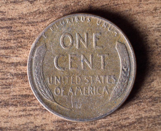
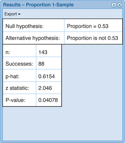
All U.S. pennies are made at either the Denver mint or the Philadelphia mint; those minted in Denver are marked with a D below the year on the face of the coin. A fast-food worker found 143 wheat pennies in the change at his restaurant; 88 of those were minted in Denver. In 2008, about 53% of all pennies were minted in Denver. Assuming that these pennies are a random sample of all wheat pennies produced, complete the hypothesis test to determine whether these data provide evidence, at the 5% level of significance, that the percentage of wheat pennies minted in Denver differs from that for all pennies minted in 2008.

- H_{0}:
- H_{a}:
- Test statistic z = (Round your answer to three decimal places.)
- Results: P-value = (Round your answer to four decimal places.)
- Conclusion: These data provide evidence to conclude that the percentage of wheat pennies minted in Denver differs from that for all pennies minted in 2008. Since the P-value our results significant at the 5% level.
Correct.

- H_{0}:p=0.53
- H_{a}:p\neq0.53
- Test statistic z=2.046
- Results: The P-value is 0.04078.
- Conclusion: These data provide strong evidence to conclude that the percentage of wheat pennies minted in Denver differs from that for all pennies minted in 2008. Since the P-value is less than 0.05, our results are significant at the 5% level.
Incorrect.

- H_{0}:p=0.53
- H_{a}:p\neq0.53
- Test statistic z=2.046
- Results: The P-value is 0.04078.
- Conclusion: These data provide strong evidence to conclude that the percentage of wheat pennies minted in Denver differs from that for all pennies minted in 2008. Since the P-value is less than 0.05, our results are significant at the 5% level.
Deciding on an appropriate level of significance is more of an art than a science. You must weigh the consequences of (incorrectly) rejecting a true null hypothesis versus those of (incorrectly) failing to reject a false null hypothesis.
8.3.2 Statistically Significant and Practically Significant

invisible clear both
Photo Credit: MANDEL NGAN/AFP/Getty Images
invisible clear both
In the previous wheat penny example, we found that our results were significant at the 5% level. This means that results at least this extreme would occur merely by chance no more than 5% of the time.
Suppose that the P-value of the penny test were 0.0498 or 0.0508 rather than 0.0408. In the first case (P-value = 0.0498) we would still say that our results are statistically significant at the 5% level, but in the second case (P-value = 0.0508), the results are not statistically significant at the 5% level. These two P-values are quite close together, differing by only 0.001, but produce opposite results when we use \alpha = 0.05. It is for this very reason that we prefer reporting the P-value, and letting the reader decide whether results are significant or not.
There is the further issue of whether results that are statistically significant have practical significance in a real world setting. With a large enough sample size, sample statistics that vary only slightly from the hypothesized value can be statistically significant, even though that difference may have little practical consequence.
During the 2008 presidential campaign, Barack Obama stated that he had promised his daughters that they could get a dog if they moved to the White House. Once Mr. Obama won the election, the media devoted a fair amount of attention to the Obamas’ search for a dog. In December 2008, the AP-Petside.com poll asked a nationally representative sample of 1129 adult pet owners whether the Obama family’s "First Dog" should be a mutt or a purebred; 19% of those interviewed thought the dog should be a purebred. Do these data provide statistically significant evidence that less than 20% of adult American dog owners believed that the Obamas should get a purebred dog?
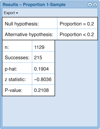
If we use CrunchIt! to perform a hypothesis test with 215 successes in a sample size of 1129, we obtain the following results.

And we see that with a P-value of 0.2108, our results are not significant, even at the \alpha = 0.10 level.
What would happen if we got the same percentage of successes, but in increasingly larger sample sizes? Below are the P-values for testing p = 0.2 against p\lt0.2 for sample sizes of 3000, 6000, and 10,000, with sample proportions of exactly 19%.
| Alternative Hypothesis | Number of Successes | Sample Size | Sample Proportion | P-Value of Test |
|---|---|---|---|---|
| p < 0.2 | 570 | 3000 | 0.19 | 0.0855 |
| p < 0.2 | 1140 | 6000 | 0.19 | 0.0264 |
| p < 0.2 | 1900 | 10,000 | 0.19 | 0.0062 |
For the very same percentage of successes, our results are significant at the 10% level with a sample size of 3000, at the 5% level with a sample size of 6000, and at the 1% level with a sample size of 10,000. This happens because there is less variability in the sampling distribution as our sample size gets larger, making the sample proportion of 0.19 more and more unusual if the population proportion were really 0.20. But regardless of the sample size, is the difference between 19% and 20% important? In this case, when we are talking about what kind of dog the First Family should get, probably not.
If you are interested in interpreting medical studies, you might want to read an extract from the article "Balancing statistical and clinical significance in evaluating treatment effects" from the Post Graduate Medical Journal. Notice that the author refers to both P-values and confidence intervals.
In situations involving drug testing or product safety, a 1% difference might be quite important. Medical researchers generally refer to practical significance as clinical significance, and require that results be both statistically significant and clinically significant. That is, they want to be sure that the results are, first of all, unlikely to have occurred merely by chance, and secondly, that these results will affect the treatment of patients.
As a consumer of statistics, you should always pay attention to both the P-value and the sample size, remembering that the larger the sample size, the more likely it is that small deviations from the hypothesized value will be statistically significant. Then you will be better able to decide about both statistical and practical or clinical significance.
8.3.3 Hypothesis Tests from Confidence Intervals
In this chapter, we used the same kind of sample data (the proportion of successes) to make two different kinds of inferences—confidence intervals and hypothesis tests. You might be curious about whether, or how, these two methods relate to one another.
In our wheat penny example, we tested whether the proportion of wheat pennies minted in Denver differed from 0.53, the proportion of 2008 pennies minted in Denver. For a sample proportion of 88/143, we rejected the null hypothesis at the \alpha = 0.05 level, based on a z-statistic of 2.046 and a P-value of 0.0408.
Using CrunchIt! to construct a 95% confidence interval for {p} using the same sample data, we find an interval of reasonable values for estimating p of 0.5356 to 0.6951. So we are 95% confident that the true proportion of wheat pennies minted in Denver lies between 0.5356 and 0.6951.
To phrase our interpretation another way, we might say that the set of likely values for p goes from 0.5356 to 0.6951. Notice that the hypothesized value of 0.53 from our hypothesis test does not lie in this interval, and thus is not a likely value for p. So our rejection of the null hypothesis that p = 0.53 at the 5% level is consistent with the values obtained for the 95% confidence interval.
Why should this be the case? Let’s recall our initial discussion of the theory underlying confidence intervals. When we select one sample at random from all the possible samples of a certain size, we calculate the sample proportion (for the characteristic being studied) for that sample. About 95% of the time, that sample proportion will be within 1.96 standard deviations of the true (but unknown) population proportion. So, 95% of the time, the true (but unknown) population proportion is within 1.96 standard deviations of whatever sample proportion we have obtained from our random sample selection. So if the hypothesized value p_{0} for a two-tailed test using a significance level of \alpha=0.05 lies within the corresponding 95% confidence interval, it is not reasonable to reject the hypothesis that p=p_{0}. On the other hand, if p_{0} is outside the interval, it is not likely that p has that value. We reject the null hypothesis, and conclude that p is different from p_{0}.
Because the P-value of our pennies test is greater than 0.01, the test is not significant at the 1% level. If we construct a 99% confidence interval, we obtain an interval ranging from 0.5106 to 0.7202. The hypothesized value of 0.53 does lie in this interval, so we are unable to conclude, at the \alpha = 1\% level, that p is different from 0.53.
Thus, we can use a (100-\alpha)\% confidence interval to draw a conclusion about a two-tailed hypothesis test at the \alpha level of significance. For a one-tailed hypothesis test, the value of \alpha represents the area of only the right- or left-hand tail, so we must use a (100-2\alpha)\% confidence interval to draw a similar conclusion about a one-tailed test. Since statistical software makes it just as easy to do a hypothesis test as a confidence interval, we are not likely to do much of this. But the fact that these inferential procedures are indeed related is an important point to make.
Our statement above, that we are unable to conclude, at the \alpha=1\% level, that p is different from 0.53 raises one more very important point about statistical significance. Sometimes statisticians phrase such a conclusion as “there is no statistically significant difference, at the 1% level, between p and 0.53.” You should not take such language to mean that there is no difference between p and 0.53; we definitely do not conclude that p is 0.53. All we can say is that we have insufficient evidence (at the indicated level) to conclude that p is a number other than 0.53.
Please review the whiteboard Connection Between a Hypothesis Test and a Confidence Interval.
8.3.4 More Accurate Confidence Intervals
Statistics, like other branches of mathematics and science, is an evolving discipline, with researchers developing new theories and techniques to improve both understanding and results. Over the past decade or two, a number of statisticians have studied the accuracy of confidence intervals for proportions, and have determined that unless the sample size is quite large, a 95% confidence interval might not capture the population proportion 95% of the time in repeated sampling. In 1998, Alan Agresti and Brent Coull published a simple fix which produces better confidence intervals for proportions when the sample size is small. (Even a sample size of several hundred might qualify, depending on the true value of p).
Here is what they discovered: adding two successes and two failures to the sample data improves accuracy for a 95% confidence interval. And that is easy enough for us to do. Returning once again to our wheat penny data, our sample had 88 successes in a sample size of 143, resulting in a 95% confidence interval for the proportion of wheat pennies minted in Denver of 0.5356 and 0.6951. Adding two successes and two failures produces an interval of 0.5335 to 0.6910.
In this instance, the improved interval is not much different from the original one, but better accuracy is always a good thing, particularly when the work to obtain it is minimal (as it is here). If you have reason to construct a confidence interval for a proportion after you finish your introductory statistics course, you might want to remember this add two successes, add two failures method.
Both confidence intervals and hypothesis tests allow us to draw conclusions about a population based on data from a single sample. We use confidence levels, P-values, and levels of significance to measure the uncertainty associated with our conclusions. When interpreting our results, or those in other studies, it is important to remember that we can never be 100% certain about any conclusions made using these techniques.