STELLAR MASSES
The final clue that astronomers needed to understand how stars work is their mass—how much matter they have. If the masses were related to the stellar luminosities and locations on the H-R diagram (which they are), then astronomers would have enough information to start making scientific models of why stars shine. The mass of each star, it turns out, determines how strongly it can compress and heat its interior and thereby create light and other electromagnetic radiation by thermonuclear fusion, which we will explore in the next chapter. Models of how stars generate that radiation, developed in the twentieth century and still being refined today, provide us with further insights into how nature works. With the knowledge gained about thermonuclear fusion in stars, physicists are researching how to control this fusion to generate electricity.
The problem with finding stellar masses is that it cannot be done directly by examining isolated stars. The mass of a star can be determined only by its gravitational effects on other bodies, using Newton’s law of gravity. When Newton derived the formula for Kepler’s third law, he discovered that for any two objects in orbit, such as a planet around the Sun, a moon around a planet, or two stars around each other, the period of their orbits is related to the sum of their masses (see Discovery 10-3: Kepler’s Third Law and Stellar Masses). You have seen in Section 2-5 that for objects orbiting the Sun, we can ignore the mass of the smaller body, thereby getting Kepler’s original third law, as stated in Chapter 2. For stars orbiting each other, we use Newton’s full equation, which includes the masses of both bodies.
Focus Question 10-9
What observations must be made to determine a star’s distance using spectroscopic parallax?
 Fortunately for astronomers, about one-third of the stars near our solar system are members of star systems in which two stars orbit each other. Put another way, about one-third of the objects we see as single stars are actually pairs of stars in orbit around each other. Most of these pairs of stars are so distant that we cannot resolve the individual stars in them with our naked eyes, and so they appear in the night sky as single objects. However, using telescopes to observe the periods of the orbits and the distances between stars, astronomers can determine the sum of the stellar masses of the pair, and as we will see shortly, they can sometimes also determine individual stellar masses.
10-10 Binary stars provide information about stellar masses
A pair of stars located at nearly the same position in the night sky is called a double star. Between 1782 and 1838, William Herschel, his sister Caroline, and his son John catalogued thousands of them. Some double stars are not physically close together and do not orbit each other. These optical doubles (sometimes called apparent binaries) just happen to lie in the same direction, as seen from Earth. For example, δ Herculis, visible with the naked eye, is an optical double with a dim star. Through a telescope these stars appear close together, but that is an optical illusion.
Other double stars are true binary stars—pairs in which two stars orbit each other. In the case of visual binaries, both stars can be seen, using a telescope if necessary (Figure 10-11). Astronomers can plot the orbit of one star around the other in a visual binary.
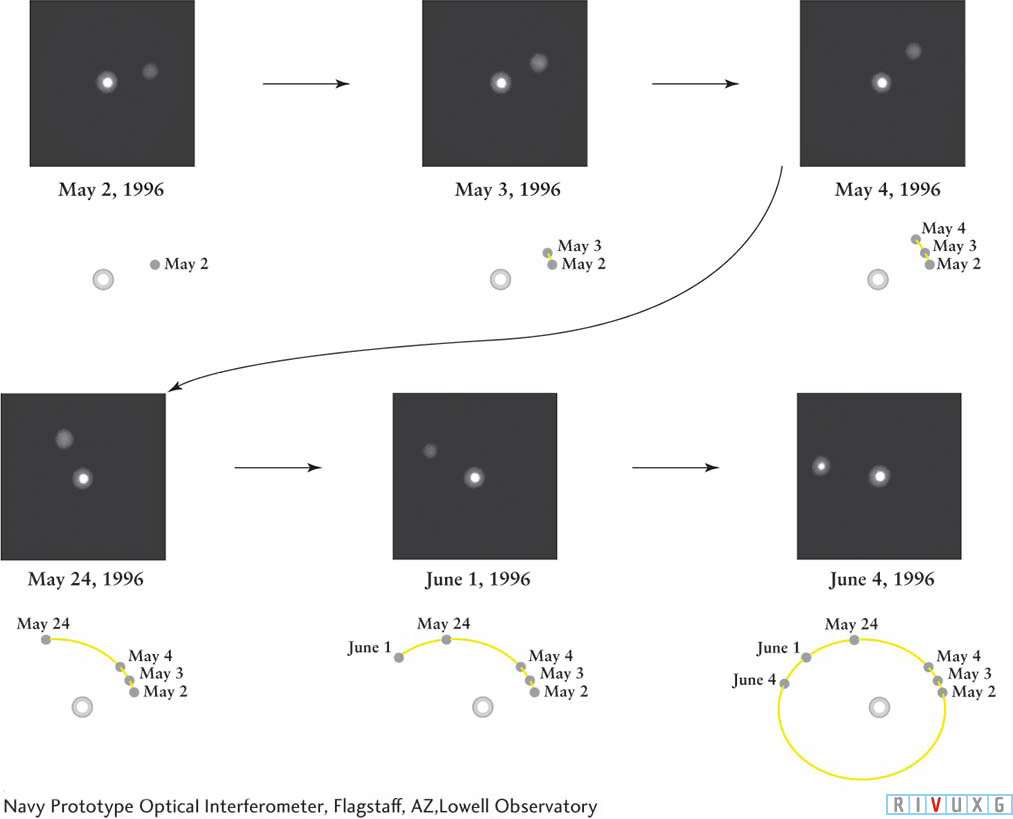
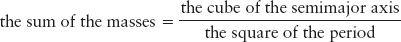
Figure 10-11  A Binary Star System About one-third of the objects we see as “stars” in our region of the Milky Way Galaxy are actually double stars. Mizar in Ursa Major is a binary system with stars separated by only about 0.01 arcsec. The images and plots show the relative positions of the two stars over nearly half of their orbital period. The orbital motion of the two binary stars around each other is evident. Either star can be considered fixed in making such plots. (Technically, this pair of stars is Mizar A and its dimmer companion. These two are bound to another binary pair, Mizar B and its dimmer companion.)
To see how we determine the masses of the individual stars, consider a visual binary. Newton rewrote Kepler’s third law as a relation between the masses of the stars (in solar masses), their orbital period around each other in Earth years (this period is the same for both stars, so it does not matter which star we assume orbits the other), and the average separation between the stars in AU (which equals the semimajor axis of the elliptical orbit):
Thus, by observing the separation between a pair of stars and how long one of them takes to complete its orbit, we can calculate the sum of the masses of the two stars, presented mathematically in Discovery 10-3: Kepler’s Third Law and Stellar Masses.
DISCOVERY 10-3
Kepler’s Third Law and Stellar Masses
The same gravitational force that holds Earth in orbit around the Sun also keeps pairs of stars in orbit around each other. For any pair of orbiting bodies, the orbits are ellipses, and Kepler’s third law can be written as
Here, M1 and M2 are the two masses (expressed in solar masses), a is the length of the semimajor axis of the ellipse (in astronomical units), and P is the orbital period (in years). Note that a is also the average separation between the two bodies. Thus, the sum of the masses can be found once we know the orbital period and average separation.
Example: Suppose two stars make up a binary system, with one star’s elliptical orbit having a semimajor axis, a, of 4 AU. We find that this star takes 2.5 years to complete one orbit. Then the sum of the stars’ masses is
M1 + M2 = (4)3/(2.5)2 = 10.2 M⊙
The total mass of the system is 10.2 M⊙.
To determine the individual masses of the stars, we need to know the distances of the stars from the center of mass of the pair. As with the Earth–Moon system discussed in Section 6-9, both stars in a binary system move in elliptical orbits around a common point between them. This point, called the center of mass, is determined by the masses of the stars and can be understood by analogy to a pair of connected masses whirling on a frictionless surface (see Figure 6-31). One point somewhere between their centers moves in a straight line. This point is the center of mass of the system of masses. Just as the two masses orbit around their center of mass, the two stars in a binary system orbit around their center of mass under the influence of their mutual gravitational attraction (Figure 10-12). The more massive star is closer to the center of mass, just as a heavier child must be closer to the pivot point or fulcrum of a seesaw for it to balance (Figure 10-12b).
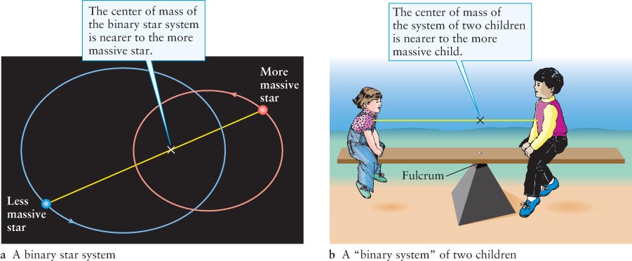
Figure 10-12 Center of Mass of a Binary Star System (a) Two stars move in elliptical orbits around a common center of mass. Although the orbits cross each other, the two stars are always on opposite sides of the center of mass and thus never collide. (b) A seesaw balances if the center of mass of the two children is at the fulcrum. When balanced, the heavier child is always closer to the fulcrum, just as the more massive star is closer to the center of mass of a binary star system.
We can locate the center of mass of a visual binary by plotting the separate orbits of the two stars, as in Figure 10-11, using the background stars as reference points. The center of mass lies at the common focus of the two elliptical orbits. To get the relative sizes of the orbits, however, we must be able to determine the plane of orbit of the two stars. This calculation is not always possible, which is why we cannot always determine the individual masses of the stars. However, when the stars in a binary system periodically eclipse each other, as seen from Earth, we know that the plane of their orbit must be nearly parallel to our line of sight to them (Figure 10-13a, b). Comparing the relative sizes of the two orbits around the center of mass yields the ratio of the two stars’ masses, M1/M2.
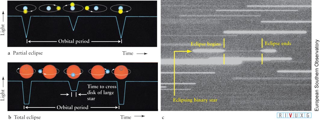
Figure 10-13
Representative Light Curves of Eclipsing Binaries The shape of the light curve (blue) reveals that the pairs of stars have orbits in planes nearly edge-on to our line of sight. It also provides details about the two stars that make up an eclipsing binary. Illustrated here are (a) a partial eclipse and (b) a total eclipse. (c) The binary star NN Serpens, indicated by the arrow, undergoes a total eclipse. The telescope was moved during the exposure so that the sky drifted slowly from left to right. During the 10.5-minute eclipse, the dimmer but larger star in the binary system (an M6 V star) passed in front of the more luminous but smaller star (a white dwarf). The binary became so dim that it almost disappeared.
When we can determine M1/M2, we can find the individual masses, because we already know the sum M1 + M2 from Kepler’s third law. The individual masses are determined by combining the ratio of the masses and the sum of the masses (that is, two equations and two unknowns yield the values for both unknowns). The range of stellar masses thus determined extends from 0.08 M⊙ to about 150 M⊙. (Stars with masses up to 265 M⊙ have been observed by other means.)
Eclipsing binaries can be detected even when the stars cannot be resolved as two distinct images in a telescope. The apparent magnitude of the image of an eclipsing binary dims each time one star blocks out part of the other. An astronomer can measure light intensity from binaries very accurately as a function of time. From these light curves, such as those shown in Figure 10-13, we can see at a glance whether the eclipse is partial, creating a V-shaped trough in the light curve (Figure 10-13a), or total, creating a flat-bottomed trough (Figure 10-13b). These data provide details of how close the plane of their orbit is to being perpendicular to our line of sight.
Light curves can also reveal information about stellar atmospheres. Suppose that one star of a binary is a tiny white dwarf (the size of Earth) and the other is a giant (much larger than the Sun). By observing exactly how the light from the white dwarf is gradually cut off as it begins to move behind the edge of the giant during an eclipse, astronomers can infer the pressure and density in the upper atmosphere of the giant. Such information is invaluable in testing models of stellar structure.
Many binary stars are separated by several astronomical units or more. Other than orbiting each other, these stars behave as though they are isolated; that is, the models we develop in the following chapters for the evolution of isolated stars apply to these binary stars as well. However, there are also close binary systems, with only a few stellar diameters separating the stars. Such stars are so close together that the gravity of each one dramatically affects the appearance and evolution of the other. If one member of a close binary is a giant, some of the gas of its outer layers is pulled onto its more compact companion—mass is transferred from one star to the other. We will explore more about such systems in Chapter 11. In addition to binary systems of stars, a few systems composed of three stars bound to each other exist in our neighborhood of space. Polaris, the North Star, for example, is part of a triple system.
10-11 Main-sequence stars have a relationship between mass and luminosity
As binary star data accumulated, an important trend began to emerge. On the main sequence, the more luminous the star, the more massive it is. This mass–luminosity relationship can be conveniently displayed graphically (Figure 10-14a); note that the axes of this figure are logarithmic. The Sun’s mass lies in the middle of both logarithmic ranges. The mass–luminosity relationship demonstrates that the main sequence on the H-R diagram is a progression in mass as well as in luminosity and surface temperature. The hot, bright, bluish stars in the upper left corner of the H-R diagram (see Figure 10-14b) are the most massive main-sequence stars. As we move down the sequence, stellar masses decrease until we reach the dim, cool, reddish stars in the lower right corner of the H-R diagram. The correlation of stellar luminosities with mass suggests (correctly, as it turns out) that a star’s energy production is closely linked to its mass. Indeed, mass is the crucial factor in explaining why stars are as bright as they are and how they evolve.
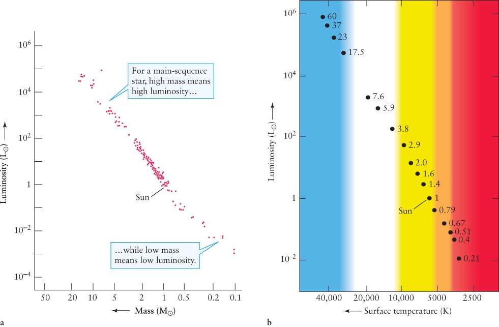
Figure 10-14 The Mass–Luminosity Relationship (a) For main-sequence stars, mass and luminosity are directly correlated—the more massive a star, the more luminous it is. A main-sequence star of mass 10 M⊙ has roughly 3000 times the Sun’s luminosity (3000 L⊙); one with 0.1 M⊙ has a luminosity of only about 0.001 L⊙. To fit the whole sequence on one page, the luminosities and masses are plotted using logarithmic scales. (b) Equivalently, on this H-R diagram, each dot represents a main-sequence star. The number next to each dot is the mass of that star in solar masses (M⊙). As you move up the main sequence from the lower right to the upper left, the mass, luminosity, and surface temperature of main-sequence stars all increase.
10-12 The orbital motion of binary stars affects the wavelengths of their spectral lines
Many binary stars are scattered throughout our Milky Way Galaxy, but only those that are nearby or are widely separated can be distinguished as visual binaries. A remote binary often presents the appearance of a single star because even our best telescopes cannot resolve the images of its individual stars. These binary systems can still be detected, however, through spectroscopy.
Spectral analysis yields incongruous spectral lines for some stars. For example, the spectrum of what appears at first to be a single star may include strong absorption lines for both hydrogen (indicating a hot, type A star) and titanium oxide (indicating a cool, type M star). Because a single star cannot display both types of absorption lines prominently, such an observation must be revealing a binary system.
Spectroscopy can also detect the movements of stars orbiting each other because of the Doppler shift in spectral lines. As we saw in Section 3-2, an approaching source of light has shorter wavelengths than if the same source were stationary, and a receding source has longer wavelengths. The amount of the shift is proportional to the speed of the light source: the greater the speed, the greater the shift.
If the two stars in a binary are orbiting at more than a few kilometers per second, they produce spectral lines that shift back and forth regularly. Such stars are called spectroscopic binaries. The motions of the stars revolving around their center of mass produce the periodic shifting of the spectral lines. In many spectroscopic binaries, one of the stars is so dim that its spectral lines cannot be detected. Instead, a single set of spectral lines from the star that we can see shifts regularly back and forth. Such a single-line spectroscopic binary yields less information about its two stars than does a double-line spectroscopic binary, in which the lines from both stars are visible. In particular, a double-line binary, in which one star eclipses the other, yields the individual masses of its two stars, whereas a single-line binary cannot provide that information.
Focus Question 10-10
For what types of stars does the mass–luminosity relationship not apply?
Figure 10-15 shows four spectra of a spectroscopic binary system. At Stage 1, star A is moving toward Earth; hence, its spectrum is blueshifted. At the same time, star B is moving away, so its spectrum is redshifted. In the spectrum below the drawing, you can see two sets of spectral lines, each slightly offset from each other. A few days later, at Stage 2, the stars have progressed along their orbits so that star A is moving toward the right and star B toward the left, as seen from Earth. Because neither star is moving toward or away from us, we see no Doppler shift and so their spectral lines return to their normal positions. Stage 3 shows the opposite spectra from Stage 1 (star A is now redshifted and star B is blueshifted), while Stage 4 shows the same spectrum as Stage 2. Figure 10-16 shows spectra taken of the binary star system κ (kappa) Arietis, demonstrating these shifts.
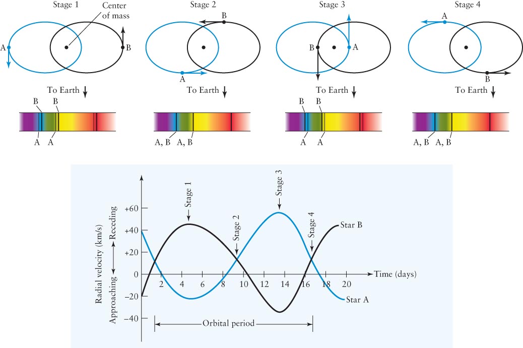
Figure 10-15 Spectral-Line Motion in Binary Star Systems The diagrams at the top indicate the positions and motions of the stars, labeled A and B, relative to Earth. Below each diagram is the spectrum we would observe for these two stars at each stage. The changes in colors (wavelengths) of the spectral lines are due to changes in the stars’ Doppler shifts, as seen from Earth. The graph displays the radial-velocity curves of the binary HD 171978. (The HD means that this is a star from the Henry Draper Catalogue of stars.) The entire binary is moving away from us at 12 km/s, which is why the pattern of radial-velocity curves is displaced upward from the zero-velocity line.
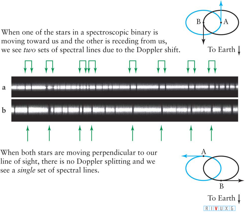
Figure 10-16
A Double-Line Spectroscopic Binary The spectrum of the double-line spectroscopic binary κ (kappa) Arietis has spectral lines that shift back and forth as the two stars revolve around each other. (a) The stars are moving parallel to the line of sight, with one star approaching Earth, the other star receding, as in Stage 1 or 3 of Figure 10-15. These motions produce two sets of shifted spectral lines. (b) Both stars are moving perpendicular to our line of sight, as in Stage 2 or 4 of Figure 10-15. As a result, the spectral lines of the two stars have merged.
The shifts in spectral lines can yield significant information about the orbital velocities of the stars in a spectroscopic binary. This information is best displayed as a radial-velocity curve, in which radial velocity is graphed over time. In Figure 10-15, the wavy pattern repeats with a period of about 15 days, which is the orbital period of the binary. This pattern is displaced upward from the zero-velocity line by about 12 km/s, which is the overall motion of the binary system away from Earth. Superimposed on this overall recessional motion are the periodic approaches and recessions of the two stars as they orbit around each other.
Combining radial-velocity curves and light curves, we can obtain other useful information from eclipsing binaries. If an eclipsing binary is also a double-line spectroscopic binary, astronomers can calculate the masses, diameters, varied brightness, speeds, and stellar separation of each star. These stars are rare, however, because the orbital planes of most spectroscopic binaries are tilted so that eclipses do not occur, as seen from Earth.
While most of the stars we see in the night sky are single objects or in binary systems, some are in groups of three or more. For example, the Pleiades in the constellation Taurus is a cluster of hundreds of stars, of which seven (the “seven sisters”) are often visible to the naked eye. Indeed, astronomers observe that many stars throughout our Milky Way Galaxy and elsewhere are found in even larger groups, which we will study in the next chapter.
Focus Question 10-11
How do the spectral lines of a spectroscopic binary change as observed from Earth?
This chapter has provided us with observational data that serve, in large measure, as the basis for the models of stellar activity and evolution presented in the next two chapters. The models make predictions that lead to new observations and refined models. As we proceed through these models, we will take up some further observations driven by these refinements.