Chapter 1. Mirror Experiment Activity 14.5
Mirror Experiment Activity 14.5
The experiment described below explored the same concepts as the one described in Figure 14.5 in the textbook. Read the description of the experiment and answer the questions below the description to practice interpreting data and understanding experimental design.
Mirror Experiment activities practice skills described in the brief Experiment and Data Analysis Primers, which can be found by clicking on the “Resources” button on the upper right of your LaunchPad homepage. Certain questions in this activity draw on concepts described in the Statistics primer. Click on the “Key Terms” buttons to see definitions of terms used in the question, and click on the “Primer Section” button to pull up a relevant section from the primer.
Experiment
Background
For the first half of the twentieth century, researchers hypothesized that mutations were changes in DNA that either occurred randomly, or were actively caused by environmental conditions. For this latter hypothesis, scientists thought that since an organism might “need” a certain trait in a particular environment, an environment could induce specific mutations that would be considered beneficial under those conditions. As you have learned in Fig. 14.5, the Lederbergs demonstrated that mutations conferring antibiotic-resistance were present in a small number of bacteria that had never been exposed to antibiotics. Thus, mutations appeared to be random events. However, it was possible that other environmental conditions, such as viruses, could induce mutations in bacteria. Are all mutations random, spontaneous events? Or can certain types of mutations be induced by specific environmental conditions?
Hypothesis
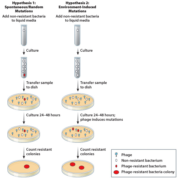
Salvador Luria and Max Delbrück grew E. coli mixed with a phage, or a virus that specifically infects bacteria. They hypothesized that if mutations conferring phage-resistance occurred randomly, different bacterial cultures would demonstrate very different numbers of phage-resistant colonies (i.e., there would be a great deal of variability). However, if mutations conferring phage-resistance were the result of bacteria being infected by phages (an environmental condition), bacterial cultures would demonstrate less variability.
Experiment
Luria and Delbrück placed non-resistant bacteria into vessels containing liquid medium. These bacteria were allowed to grow, and if mutations actually occurred randomly, some phage-resistant bacteria would be present in liquid cultures at the end of the incubation period. Samples from these liquid cultures were then transferred to dishes containing an E. coli phage. After 24-48 hours of culture, researchers counted the number of phage-resistant colonies present in each dish (Figure 1). Using mathematical equations, researchers were able to determine how much the number of phage-resistant bacterial colonies varied from culture to culture.
Results
Luria and Delbrück determined that there was a great deal of variability in the number of phage-resistant bacterial colonies observed in dishes containing the phage. Some cultures contained no phage-resistant colonies, while other cultures contained dozens (or even hundreds). This work provided evidence that mutations conferring phage-resistance in bacteria occurred randomly and independently of environmental conditions.
Source
Luria, S. E., Delbruck, M., 1943. Mutations of Bacteria from Virus Sensitivity to Virus Resistance. Genetics. 28, 491-511.

Question
In order to determine the variation in the number of phage-resistant colonies present in different cultures, Luria and Delbrück calculated a statistical value known as the variance. In order to calculate the variance of a data set, researchers must first determine the mean of their data. For example, if a researcher measured three individuals and determined that their heights were 50 inches, 70 inches and 60 inches, the mean of this data set would be 60 inches (i.e., (50+70+60)/3). Imagine that for one of their experiments, Luria and Delbrück found the following numbers of phage-resistant colonies in five different cultures: 0, 17, 58, 23, and 47. What is the mean number of phage-resistant colonies for this data set?
| A. |
| B. |
| C. |
| D. |
| E. |
| Variance | The square of the standard deviation. |
| Standard deviation | The extent to which most of the measurements are clustered near the mean. To obtain the standard deviation, you calculate the difference between each individual measurement and the mean, square the difference, add these squares across the entire sample and divide by n – 1, and take the square root of the result. |
| Mean | The arithmetic average of all the measurements (all the measurement added together and the result divided by the number of measurements); the peak of a normal distribution along the x-axis. |
From the Statistics primer
The Normal Distribution

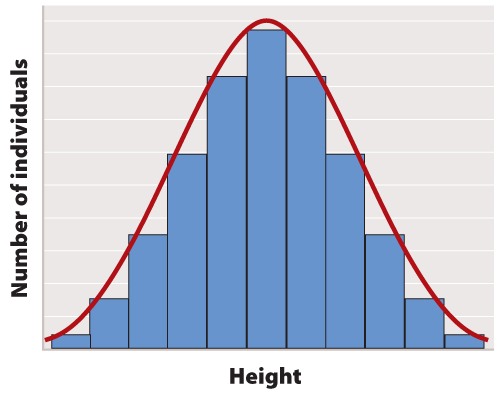
The first step in statistical analysis of data is usually to prepare some visual representation. In the case of height, this is easily done by grouping nearby heights together and plotting the result as a histogram like that shown in Figure 1. The smooth, bell-shaped curve approximating the histogram in Figure 1A is called the normal distribution. If you measured the height of more and more individuals, then you could make the width of each bar in the histogram narrower and narrower, and the shape of the histogram would gradually get closer and closer to the normal distribution.

The normal distribution does not arise by accident but is a consequence of a fundamental principle of statistics which states that when many independent factors act together to determine the magnitude of a trait, the resulting distribution of the trait is normal. Human height is one such trait because it results from the cumulative effect of many different genetic factors as well as environmental effects such as diet and exercise. The cumulative effect of the many independent factors affecting height results in a normal distribution.
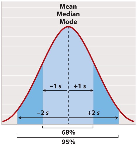
The normal distribution appears in countless applications in biology. Its shape is completely determined by two quantities. One is the mean, which tells you the location of the peak of the distribution along the x-axis (Figure 2). While we do not know the mean of the population as a whole, we do know the mean of the sample, which is equal to the arithmetic average of all the measurements—the value of all of the measurements added together and divided by the number of measurements.
In symbols, suppose we sample n individuals and let xi be the value of the ith measurement, where i can take on the values 1, 2, ..., n. Then the mean of the sample is given by , where the symbol means “sum” and means x1 + x2 + ... + xn.
For a normal distribution, the mean coincides with another quantity called the median. The median is the value along the x-axis that divides the distribution exactly in two—half the measurements are smaller than the median, and half are larger than the median. The mean of a normal distribution coincides with yet another quantity called the mode. The mode is the value most frequently observed among all the measurements.
The second quantity that characterizes a normal distribution is its standard deviation (“s” in Figure 2), which measures the extent to which most of the measurements are clustered near the mean. A smaller standard deviation means a tighter clustering of the measurements around the mean. The true standard deviation of the entire population is unknown, but we can estimate it from the sample as
What this complicated-looking formula means is that we calculate the difference between each individual measurement and the mean, square the difference, add these squares across the entire sample, divide by n - 1, and take the square root of the result. The division by n - 1 (rather than n) may seem mysterious; however, it has the intuitive explanation that it prevents anyone from trying to estimate a standard deviation based on a single measurement (because in that case n - 1 = 0).
In a normal distribution, approximately 68% of the observations lie within one standard deviation on either side of the mean (Figure 2, light blue), and approximately 95% of the observations lie within two standard deviations on either side of the mean (Figure 2, light and darker blue together). You may recall political polls of likely voters that refer to the margin of error; this is the term that pollsters use for two times the standard deviation. It is the margin within which the pollster can state with 95% confidence the true percentage of likely voters favoring each candidate at the time the poll was conducted.

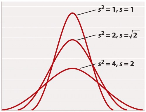
For reasons rooted in the history of statistics, the standard deviation is often stated in terms of s2 rather than s. The square of the standard deviation is called the variance of the distribution. Both the standard deviation and the variance are measures of how closely most data points are clustered around the mean. Not only is the standard deviation more easily interpreted than the variance (Figure 2), but also it is more intuitive in that standard deviation is expressed in the same units as the mean (for example, in the case of height, inches), whereas the variance is expressed in the square of the units (for example, inches2). On the other hand, the variance is the measure of dispersal around the mean that more often arises in statistical theory and the derivation of formulas. Figure 3 shows how increasing variance of a normal distribution corresponds to greater variation of individual values from the mean. Since all of the distributions in Figure 3 are normal, 68% of the values lie within one standard deviation of the mean, and 95% within two standard deviations of the mean.
Another measure of how much the numerical values in a sample are scattered is the range. As its name implies, the range is the difference between the largest and the smallest values in the sample. The range is a less widely used measure of scatter than the standard deviation.

