EXAMPLE 7 Bonferroni method of multiple comparisons
Use the Bonferroni method of multiple comparisons to determine which pairs of population mean times differ, for the mice in Groups 0, 1, and 2 in Example 5. Use level of significance .
Solution
The Bonferroni method requires that
- the requirements for ANOVA have been met, and
- the null hypothesis that the population means are all equal has been rejected.
In Example 5, we verified both requirements.
Step 1 For each of the c hypothesis tests, state the hypotheses and the rejection rule. There are means, so there will be hypothesis tests. Our hypotheses are
- Test 1:
- Test 2:
- Test 3:
where represents the population mean time spent in the open-ended sections of the maze, for the th group. For each hypothesis test, reject if the Bonferroni-adjusted .
Step 2 Calculate for each hypothesis test. From Figure 11 on page 676, we have the mean square error from the original ANOVA as MSE = 52.9485079 and from Figure 21 we get the sample means and the sample sizes. Thus,
- Test 1:
- Test 2:
- Test 3:
When the requirements are met, follows a distribution with degrees of freedom, where represents the total sample size.
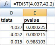
 Figure 12.22: FIGURE 22 Unadjusted -values from Excel.
- Test 1:
- Step 3 Find the Bonferroni-adjusted -value for each hypothesis test. Figure 22 shows the unadjusted -values for the values of from Step 2, using the function tdist , where and the 2 represents a two-tailed test. Then the Bonferroni-adjusted , for each hypothesis test.
688
- Test 1: Bonferroni-adjusted .
- Test 2: Bonferroni-adjusted .
- Test 3: Bonferroni-adjusted , but this value exceeds 1, so we set this -value equal to 1.
- Step 4 For each hypothesis test, state the conclusion and the interpretation.
- Test 1: The adjusted , which is ≤0.01; therefore, reject . There is evidence at the 0.01 level of significance that the population mean time spent in the open-ended part of the maze differs between Group 0 and Group 1.
- Test 2: The adjusted , which is ≤0.01; therefore, reject . There is evidence at the 0.01 level of significance that the population mean time differs between Group 0 and Group 2.
- Test 3: The adjusted , which is not ≤0.01; therefore, do not reject . There is insufficient evidence at the 0.01 level of significance that the population mean time differs between Group 1 and Group 2.
NOW YOU CAN DO
Exercises 9–18.