EXAMPLE 15 Dummy variables in multiple regression
- Verify that the regression assumptions are met.
- Perform a multiple regression of on and , using level of significance . Find the two regression equations, one for females and the other for males.
- Construct a scatterplot of versus , using different-shaped points to show the different sexes. Place the two regression equations on the scatterplot.
- Interpret the coefficient of the dummy variable .
Solution
Figures 26 and 27 contain no evidence of unhealthy patterns. We therefore conclude that the regression assumptions are verified.
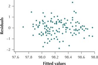 Figure 13.27: FIGURE 26 Scatterplot of residuals versus fitted values.
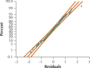 Figure 13.28: FIGURE 27 Normal probability plot of the residuals.
750
- Figure 28 contains the multiple regression results. The -value for the test is 0.001, which is , so we conclude that the overall regression is significant. The regression results tell us that , , and . Thus, our two regression equations are:
- Females:
- Males:
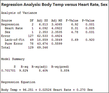 Figure 13.29: FIGURE 28 Results for multiple regression of on and .
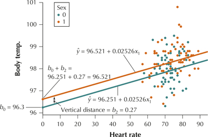 Figure 13.30: FIGURE 29 Scatterplot showing parallel regression lines when using dummy variables.
 - Figure 29 contains the scatterplot of versus , with the orange dots representing females and the blue dots representing males. The regression lines are shown, orange for females, blue for males. Note that the regression lines are parallel, because they each have the same slope . So the only difference in the lines is the intercepts.
- For females, the intercept is .
- For males, the intercept is simply .
- The vertical distance between the parallel regression lines equals , as shown in Figure 29. Thus, we interpret the coefficient of the dummy variable as the estimated increase in for those observations with (females), as compared to those with (males), when heart rate is held constant. That is, for the same heart rate, females have a body temperature that is higher than that of males, by an estimated 0.27 degrees.
NOW YOU CAN DO
Exercise 29.