Example 16

EXAMPLE 16 Strategy for building a multiple regression model

baseball2013

The author of this book first became interested in the field of statistics through the enjoyment of sports statistics, especially baseball, which is packed with interesting statistics. Today, professional sports teams are seeking competitive advantage through the analysis of data and statistics, such as Sabermetrics (Society of American Baseball Research, www.sabr.org), as shown in the motion picture Moneyball.

Suppose a baseball researcher is interested in predicting $y = runs scored$ , using the data set Baseball 2013 and the following predictor variables:

$x_{1} = Hits, the number of hits (of all kinds) the player makes$
$x_{2} = Doubles, the number of doubles the player makes$
$x_{3} = Triples, the number of triples the player makes$
$x_{4} = Home Runs, the number of home runs the player makes$
$x_{5} = RBIs, the number of runs batted in (runs scored by other players, but caused by this player)$
$x_{6} = Walks, the number of walks issued to the player$
$x_{7} = Batting Average, the number of hits divided by the number of at-bats$
$x_{8} = Red Sox, a dummy variable equal to 1 if the player plays for the Boston Red Sox, and 0 otherwise$

Use the Strategy for Building a Multiple Regression Model to build the best multiple regression model for predicting the number of runs scored using these predictor variables, at level of significance $α = 0.05$ .

Solution

The data set Baseball 2013 contains the batting statistics of the $n = 448$ players in Major League Baseball who had at least 100 at-bats during the 2013 season (Source: www.seanlahman.com/baseball-archive/statistics).

Step 1 The $F$ Test. Figure 30 shows the Minitab results of a regression of $y = runs scored$ on the set of predictor variables $x_{1}, x_{2}, x_{3}, \dots, x_{8}$ . The $p$ -value for the $F$ test is significant, so we know that a linear relationship exists between $y = runs scored$ and at least one of the $x$ variables.
Step 2 The $t$ test (the first time). In Figure 30, the $p$ -value for Batting Average is greater than level of significance $α = 0.05$ . We therefore eliminate the Batting Average from the model. Perhaps surprisingly, a player's batting average is evidently not helpful in predicting the number of runs that player will score when all other predictors are held constant.

Page 752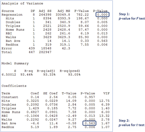

FIGURE 30 Step 1: $F$ test is significant.

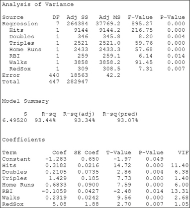FIGURE 31 All $x$ variables are significant; we have our final model.
Step 2 The $t$ test (the second time). We repeat Step 2 as long as there are $x$ variables with $p$ -values greater than level of significance $α = 0.05$ . Figure 31 shows the results of performing the multiple regression of $y = Runs Scored$ on all the $x$ variables except Batting Average. No further variables have $p$ -values below 0.05; therefore, no further variables are excluded from the model. In other words, we have our final model.
Step 3 Verify the assumptions. For our final model, we now verify the regression assumptions. Figures 32 and 33 show no patterns for the bulk of the data that would indicate a violation of the regression assumptions. We therefore conclude that the regression assumptions are verified.

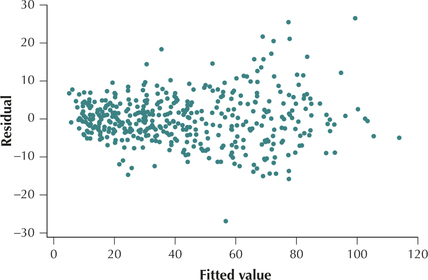FIGURE 32 Scatterplot of residuals versus fitted values.

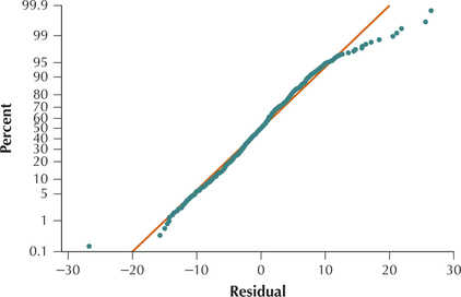FIGURE 33 Normal probability plots of the residuals.
Step 4 Report and interpret your final model.
1. The multiple regression equation for the final model is shown here.
  
  $\begin{array}{l} \hat{y} = & - 1.283 + 0.3182 Hits + 0.2105 Doubles + 1.429 Triples + 0.6833 Home Runs \\ - 0.1059 RBIs + 0.2319 Walks + 5.08 Red Sox \end{array}$
  
  Page 753
2. We interpret the coefficient for Hits, and leave to the exercises the interpretation of the other multiple regression coefficients. “For each additional hit that a player makes, the estimated increase in the number of runs that player will score is 0.3182, when all the other $x$ variables are held constant.”
3. The standard error of the estimate for the final model is $s = 6.4952 \approx 6.5$ . That is, using the multiple regression equation in (a), the size of the typical prediction error will be about 6.5 runs. The value of the adjusted coefficient of determination is $R_{adj}^{2} = 93.07 %$ . In other words, 93.07% of the variability in the number of runs scored is accounted for by this multiple regression equation.

NOW YOU CAN DO

Exercises 24–26 and 31–33.