EXAMPLE 26 Using the runs test for linear regression
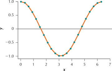
Consider the following ordered bivariate data set and the accompanying scatterplot (Figure 27). We are interested in performing linear regression of the variable on the variable. Make a scatterplot of the residuals versus the fts . Classify the residuals as being either positive (P) or negative (N). Then evaluate the independence assumption for the linear regression model by performing the runs test for randomness on the residuals, ordered by the fits.
| 0.0 | 1.00000 | 3.3 | −0.98748 |
| 0.3 | 0.95534 | 3.6 | −0.89676 |
| 0.6 | 0.82534 | 3.9 | −0.72593 |
| 0.9 | 0.62161 | 4.2 | −0.49026 |
| 1.2 | 0.36236 | 4.5 | −0.21080 |
| 1.5 | 0.07074 | 4.8 | 0.08750 |
| 1.8 | −0.22720 | 5.1 | 0.37798 |
| 2.1 | −0.50485 | 5.4 | 0.63469 |
| 2.4 | −0.73739 | 5.7 | 0.83471 |
| 2.7 | −0.90407 | 6.0 | 0.96 017 |
| 3.0 | −0.98999 | 6.3 | 0.99986 |

14-60
Solution
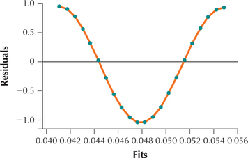
The scatterplot of the residuals versus the fts is shown in Figure 28.

What Results Might We Expect?
When applied to linear regression analysis, the runs test for randomness tests whether a pattern exists in the residuals. Do you observe a pattern in the scatterplot of the residuals (Figure 28)? If so, then what might we expect our conclusion to be for the runs test? Yes, there appears to be a descending and then ascending pattern in the data (In fact, can you discern the exact relationship between and ?), and thus we expect to reject the null hypothesis that the data are random
By examining Figure 28, we can classify the residuals from left to right as positive or negative, giving us:
| P | P | P | P | P | P | N | N | N | N | N | N | N | N | N | N | P | P | P | P | P | P |
The residuals are ordered by the size of the fts, and we have classified each residual into one of two distinct outcomes. Thus, we may proceed with the hypothesis test.
- Step 1 State the hypotheses.
- Step 2 Find the critical values, and state the rejection rule. We have positives and negatives, so the small-sample case applies ( and ). From Appendix Table L we find our critical values and . We will reject if or if .
- Step 3 Find the value of the test statistic. We have the small-sample case, so the test statistic is simply the number of runs, :
- Step 4 State the conclusion and the interpretation. Because is less than 7, we reject . Evidence exists that the sequence of residuals is not random. The residuals are nonrandom, so the independence assumption for the linear regression model is violated, and we should not proceed with a linear regression analysis.
By the way, have you guessed the equation of the pattern shown in Figures 27 and 28? The relationship between and is .