EXAMPLE 25 Constructing a time series plot using technology

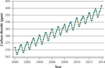
The data set Mauna Loa 1 contains the carbon dioxide levels at Mauna Loa from May 2000 to May 2014. Use technology to construct a time series plot of the data.

Solution

We use the instructions provided in the Step-by-Step Technology Guide at the end of this section. The resulting Minitab time series plot is shown in Figure 49. (The year on the horizontal axis indicates the month of May of each year. For example “2014” refers to May 2014.)

In Figure 49, we observe both a seasonal pattern and a long-term trend. Every autumn and winter, the carbon dioxide level increases, and every summer it decreases. In autumn and winter, leaves and other deciduous vegetation decay, releasing their store of carbon back into the atmosphere. In the spring and summer, the new year's leaves require carbon to grow and extract it from the atmosphere, thereby reducing the atmosphere's carbon dioxide level. Thus, the biosphere “inhales” carbon each summer and “exhales” it each winter. However, the low point of each successive cycle does not quite reach the level of the previous cycle before heading up again. This leads to an overall increasing trend in the amount of carbon dioxide in the atmosphere as we move from 2000 to 2014.

91