Example 10

EXAMPLE 10 Calculating and interpreting prediction errors (residuals)

Use the regression equation from Example 9 to calculate and interpret the prediction error (residual) for the following cities.

Solution

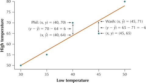
The actual data point for Philadelphia is shown in the scatterplot in Figure 27 (denoted as “Phil”). In Example 9, we calculated the predicted high temperature for Philadelphia to be $\hat{y} = 64 ° F$ . In Figure 27, $\hat{y} = 64 ° F$ represents the $y$ -value of the point on the regression line where it intersects $x = 40 ° F$ . That is, the actual high temperature $y = 70 ° F$ lies directly above predicted temperature $\hat{y} = 64 ° F$ for low temperature $x = 40 ° F$ .
The actual high temperature in Washington that day was $y = 65$ . Using the regression equation, the predicted high temperature is $\hat{y} = 1.4 (45) + 8 = 71$ . So the prediction error is $y - \hat{y} = 65 - 71 = - 6 ° F$ . The data point lies below the regression line, so that its actual high temperature of 65°F is lower than predicted given its low temperature of 45°F.

Philadelphia, Pennsylvania

Page 215

FIGURE 27 Prediction error for Philadelphia and Washington, DC.

NOW YOU CAN DO

Exercises 25b–36b.