EXAMPLE 2 Constructing a scatterplot
sqrfootsale
Suppose you are interested in moving to Glen Ellyn, Illinois, and want to purchase a lot upon which to build a new house. Table 1 contains a random sample of eight lots for sale in Glen Ellyn, with their square footage and prices.
- Identify the predictor variable and the response variable.
- Construct a scatterplot.
| Lot | ||
|---|---|---|
| Harding St. | 75 | 155 |
| Newton Ave. | 125 | 210 |
| Stacy Ct. | 125 | 290 |
| Eastern Ave. | 175 | 360 |
| Second St. | 175 | 250 |
| Sunnybrook Rd. | 225 | 450 |
| Ahlstrand Rd. | 225 | 530 |
| Eastern Ave. | 275 | 635 |
Note: The square footage is expressed in 100s of square feet, so that “90” represents square feet. Similarly, the sales price is expressed in $1000s, so that .
Solution
- It is reasonable to expect that the price of a new lot depends in part on the size of the lot. Thus, we define our predictor variable to be and our response variable to be .
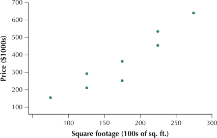
- Next, we construct the scatterplot using the data from Table 1. Draw the horizontal axis so that it can contain all the values of the predictor variable, and similarly for the vertical axis. Then, at each data point , draw a dot. For example, for the Harding Street lot, move along the x axis to 75, then go up until you reach a spot level with , at which point you draw a dot. Proceed similarly for the other seven properties. The result should look similar to the scatterplot in Figure 1.
 Figure 4.1: FIGURE 1 Scatterplot of sales price versus square footage.
190
From this scatterplot, we can see that larger lots tend to have higher prices. This is not the case for each observation. For example, the Second Street property is larger than the Stacy Court property, but it has a lower price. Nevertheless, the overall tendency remains.
NOW YOU CAN DO
Exercises 13a–20a.