Example 14

EXAMPLE 14 The $p$ -value method using technology: Two-tailed test

brisbane

The birth weights, in grams (1000 grams = 1 kilogram ≈ 2.2 pounds), of a random sample of 44 babies from Brisbane, Australia, have a sample mean weight $\bar{x} = 3276 grams$ . Formerly, the mean birth weight of babies in Brisbane was 3200 grams. Assume that the population standard deviation $σ = 528$ grams. Is there evidence that the population mean birth weight of Brisbane babies now differs from 3200 grams? Use technology to perform the appropriate hypothesis test, with level of significance $α = 0.10$ .

What Results Might We Expect?

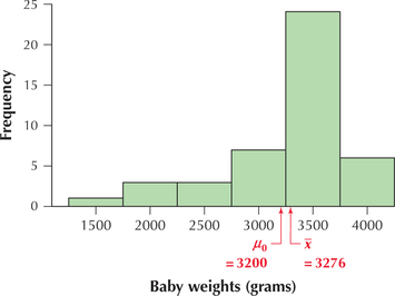
Note from Figure 8 that the sample mean birth weight $\bar{x} = 3276$ grams is close to the hypothesized mean birth weight of $μ_{0} = 3200$ grams. This value of $\bar{x}$ is not extreme and thus does not seem to offer strong evidence that the hypothesized mean birth weight is wrong. Therefore, we might expect to not reject the hypothesis that $μ_{0} = 3200$ grams.

FIGURE 8 Sample mean,

$\bar{x} = 3276$ , is close to hypothesized mean,

$μ_{0} = 3200$ , so we expect to not reject the null hypothesis.

Solution

The sample size $n = 44$ is large and $σ = 528$ is known, so we may proceed with the $Z$ test for $μ$ .

Step 1 State the hypotheses and the rejection rule.

The key words “differs from” mean that we have a two-tailed test:

$H_{0} : μ = 3200 versus H_{a} : μ \neq 3200$

where $μ$ refers to the population mean birth weight of Brisbane babies. We will reject $H_{0}$ if the $p -value \leq α = 0.10$ .
Step 2 Calculate $Z_{data}$ .

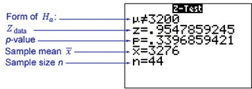
We will use the instructions provided in the Step-by-Step Technology Guide at the end of this section (page 519). Figure 9 shows the TI-83/84 results from the $Z$ test for $μ$ :

FIGURE 9 TI-83/84 results.

Page 513

$Z_{data} = \frac{\bar{x} - μ_{0}}{σ / \sqrt{n}} = \frac{3276 - 3200}{528 / \sqrt{44}} = 0.9547859245 \approx 0.9548$

Figure 10 shows the Minitab results, where

“Test of $μ = 3200$ versus ≠ 3200” refers to the hypotheses being tested, $H_{0} : μ = 3200$ versus $H_{a} : μ \neq 3200$ .
“The assumed standard deviation = 528” refers to our assumption that $σ = 528$ .
SE Mean refers to the standard error of the mean, that is, $σ / \sqrt{n}$ . You can see that $528 / \sqrt{44} \approx 79.6$ .
90% CI represents a 90% $Z$ confidence interval for $μ$ .
$Z$ refers to our test statistic:

$Z_{data} = \frac{\bar{x} - μ_{0}}{σ / \sqrt{n}} = (3276 - 3200) / (528 / \sqrt{44}) = 0.9547859245 \approx 0.95$
$P$ represents our $p$ -value of 0.340.

FIGURE 10 Minitab results.

Different software rounds the results to different numbers of decimal places.

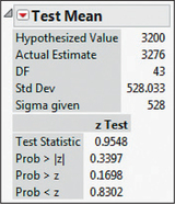
Figure 11 shows the JMP results, where

FIGURE 11 JMP results.

“Hypothesized Value” refers to the hypotheses being tested: $H_{0} : μ = 3200$ versus $H_{a} : μ \neq 3200$ .
“Actual Estimate” refers to the sample mean, $\bar{x} = 3276$ .
“Sigma given” refers to our assumption that $σ = 528$ .
“Test statistic” refers to $Z_{data}$ , our test statistic.
“ $Prob > | z |$ ,” “ $Prob > z$ ,” and “ $Prob < z$ ” refers to the $p$ -value of a two-sided, right-tailed, and left-tailed test, respectively. We want the two-sided $p$ -value, which is $“ Prob > | z | ” = 0.3397$ .

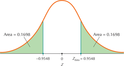
Step 3 Find the $p$ -value.

We have a two-tailed test from Step 1, so that from Table 5 our $p$ -value is (Figure 12)

$\begin{matrix} p -Value = 2 \cdot P (Z > | Z_{data} |) = 2 \cdot P (Z > 0.9548) \approx 2 \cdot (0.1698) \\ = 0.3396 \end{matrix}$

FIGURE 12 $p$ -Value is the sum of two tail areas: $0.1698 + 0.1698 = 0.3396$ .

Page 514
Step 4 State the conclusion and interpretation.

Because 0.3396 is not ≤ 0.10, we do not reject $H_{0}$ . There is insufficient evidence that the population mean birth weight differs from 3200 grams. This conclusion is just as we expected.

NOW YOU CAN DO

Exercises 27–30.