Chapter 13 Review Exercises
section 13.1
For Exercises 1–3, test whether a linear relationship exists between x and y, using level of significance α=0.05.
Question 13.145
eduearn
1. Education and Earnings. The U.S. Census Bureau reports the mean annual earnings of American citizens according to the number of years of education. We are interested in the relationship between earnings (y, in thousands of dollars) and years of education (x).
| Education (x) | Annual earnings (y) |
|---|---|
| 8 | 18.6 |
| 10 | 18.9 |
| 12 | 27.3 |
| 13 | 29.7 |
| 14 | 34.2 |
| 16 | 51.2 |
| 18 | 60.4 |
13.99.1
H0:β1=0: There is no linear relationship between Education (x) and Annual Earnings (y). Ha:β1≠0: There is a linear relationship between Education (x) and Annual Earnings (y). Reject H if tdata≥2.571 or tdata≤−2.571 . Since tdata=7.542≥2.571, we reject H0. There is evidence at level of significance α=0.05 that β1≠0 and that there is a linear relationship between Education (x) and Annual Earnings (y).
Question 13.146
gpa
2. High School GPA and College GPA. The college admissions office wants to determine if a relationship exists between the high school grade point average (x) and the grade point average of first-year college students (y), using the data in the following table.
| Student | High school GPA (x) |
First-year college GPA (y) |
|---|---|---|
| 1 | 2.4 | 2.6 |
| 2 | 2.5 | 1.9 |
| 3 | 2.9 | 2.7 |
| 4 | 2.7 | 2.5 |
| 5 | 3.0 | 2.4 |
| 6 | 3.5 | 2.9 |
| 7 | 3.0 | 2.7 |
| 8 | 3.6 | 3.1 |
| 9 | 3.4 | 3.0 |
| 10 | 3.9 | 3.3 |
Question 13.147
ageprice
3. Used Cars: Price versus Age. Do you think you can predict the price of a used car based on how old it is? The table shows the age (x, in years) and the price (y, in thousands of dollars) of 10 previously owned vehicles of the same make and model.
| Car | Age (x) |
Price (y) |
|---|---|---|
| 1 | 1 | 18.0 |
| 2 | 2 | 16.0 |
| 3 | 3 | 15.5 |
| 4 | 4 | 13.5 |
| 5 | 4 | 14.5 |
| 6 | 5 | 10.5 |
| 7 | 5 | 12.0 |
| 8 | 6 | 9.5 |
| 9 | 7 | 8.5 |
| 10 | 8 | 7.0 |
13.99.3
H0:β1=0: There is no linear relationship between Age (x) and Price Ha:β1≠0: There is a linear relationship between Age (x) and Price (y). Reject H0 if tdata≥2.306 or tdata≤−2.306. Since tdata=−15.0124≤−2.306, we reject H0. There is evidence at level of significance α=0.05 that β1≠0 and that there is a linear relationship between Age (x) and Price (y).
For Exercises 4–6, construct and interpret a 95% confidence interval for β1
Question 13.148
4. Data in Exercise 1
Question 13.149
5. Data in Exercise 2
13.99.5
(0.339, 1.029). We are 95% confident that the interval (0.339, 1.029) captures the population slope b1 of the relationship between high school GPA and first-year college GPA.
Question 13.150
6. Data in Exercise 3
section 13.2
For Exercises 7–9, do the following, for the indicated data:
- Find the point estimate of y, for the given x.
- Calculate and interpret a 95% confidence interval for the mean value of y for the given x.
- Compute and interpret a 95% prediction interval for a randomly chosen value of y for the given x.
Question 13.151
7. Data in Exercise 1, for 10 years of education
13.99.7
(a) 20.92 thousand dollars (b) (14.28, 27.56). We are 95% confident that the mean annual salary for people with 10 years of education lies between 14.28 thousand dollars and 27.56 thousand dollars. (c) (6.55, 35.29). We are 95% confident that the annual salary for a randomly selected person with 10 years of education lies between 6.55 thousand dollars and 35.29 thousand dollars.
Question 13.152
8. Data in Exercise 2, for a high school GPA of 3.0
Question 13.153
9. Data in Exercise 3, for a used car that is eight years old
13.99.9
(a) 6.818 thousand dollars (b) (5.805, 7.831). We are 95% confident that the mean price for 8-year-old cars of this make and model lies between 5.805 thousand dollars and 7.831 thousand dollars (c) (4.902, 8.733). We are 95% confident that the price for a randomly selected 8-year-old car of this make and model lies between 4.902 thousand dollars and 8.733 thousand dollars.
section 13.3
Use the following data set for Exercises 10–13.
| y | x1 | x2 | x3 |
|---|---|---|---|
| 18.7 | 2 | 100 | 4.1 |
| 18.4 | 4 | 90 | 5.0 |
| 21.8 | 6 | 90 | 3.8 |
| 22.0 | 8 | 70 | 5.2 |
| 25.2 | 10 | 70 | 3.8 |
| 25.7 | 12 | 50 | 5.3 |
| 26.9 | 14 | 50 | 5.4 |
| 28.3 | 16 | 30 | 5.4 |
| 28.6 | 18 | 30 | 4.3 |
| 31.8 | 20 | 10 | 4.9 |
Question 13.154
10. Assume the regression assumptions are met. Perform the F test for the significance of the overall regression, using level of significance α=0.05. Do the following:
- State the hypotheses and the rejection rule.
- Find the F statistic and the p-value.
- State the conclusion and interpretation.
Question 13.155
11. Perform the t test for the significance of the individual predictor variables, using level of significance α=0.05. Do the following:
- For each hypothesis test, state the hypotheses and the rejection rule.
- For each hypothesis test, find the t statistic and the p-value.
- For each hypothesis test, state the conclusion and interpretation.
13.99.11
(a) Test 1:H0:β1=0: There is no linear relationship between y and x1. Ha:β1≠0: There is a linear relationship between y and x1. Reject H0 if the p-value ≤α=0.05. Test 2:H0:β2=0: There is no linear relationship between y and x2. Ha:β2≠0: There is a linear relationship between y and x2. Reject H0 if the p-value ≤α=0.05. Test 3:H0:β3=0: There is no linear relationship between y and x3. Ha:β3≠0: There is a linear relationship between y and x3. Reject H0 if the p-value ≤α=0.05. (b) Test 1:t=1.86, with p-value=0.112; Test 2:t=−0.27, with p-value=0.798; Test 3: t=−1.07, with p-value=0.326. (c) Test 1: The p-value=0.112, which is not ≤α=0.05. Therefore we do not reject H0. There is insufficient evidence of a linear relationship between y and x1. Test 2: The p-value=0.798, which is not ≤α=0.05. Therefore we do not reject H0. There is insufficient evidence of a linear relationship between y and x2. Test 3: The p-value=0.326, which is not ≤α=0.05. Therefore we do not reject H0. There is insufficient evidence of a linear relationship between y and x3.
Question 13.156
12. Identify any predictors that have corresponding p-values greater than the level of significance α=0.05. Of these, discard the variable with the largest p-value. Then redo Exercise 11, omitting this predictor. Repeat if necessary.
Question 13.157
13. Verify the regression assumptions for your final model from Exercise 12.
13.99.13
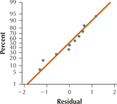
The preceding scatterplot of the residuals versus fitted values shows no strong evidence of unhealthy patterns. Thus, the independence assumption, the constant variance assumption, and the zero-mean assumption are verified. Also, the normal probability plot of the residuals indicates no evidence of departure from normality of the residuals. Therefore we conclude that the regression assumptions are verified.