Section 3.1 Exercises
CLARIFYING THE CONCEPTS
Question 3.1
1. Explain what a measure of center is. (p. 108)
3.1.1
A value that locates the center of the data set.
Question 3.2
2. Which measure may be used as the balance point of the data set? Explain how this works. (p. 110)
Question 3.3
3. Explain what we mean when we say that the mean is sensitive to the presence of extreme values. Explain whether the median is sensitive to extreme values. (pp. 111-112)
3.1.3
Because the mean depends in part on the sum of all data values, an outlier will skew the mean (pull it in one direction or another). Since the median simply depends on position in an ordered list, it is not sensitive to outliers.
Question 3.4
4. What are the three measures of center that we learned about in this section? (p. 108)
For Exercises 5–12, either state what is being described or provide the notation.
Question 3.6
6. The number of observations in your population data set (p. 109)
Question 3.8
8. Notation for what we get when we add up all the data values in the population, and divide by how many observations there are in the population (p. 109)
Question 3.9
9. Notation for what we get when we add up all the data values in the sample, and divide by how many observations there are in the sample (p. 109)
3.1.9
ˉx
Question 3.10
10. The middle data value when the data are put in ascending order (p. 112)
Question 3.12
12. The sample mean (p. 109)
PRACTICING THE TECHNIQUES
 CHECK IT OUT!
| To do | Check out | Topic |
|---|---|---|
| Exercises 13–18 | Example 1 | Population mean |
| Exercises 19–24 | Example 2 | Sample mean |
| Exercises 25–30 | Example 3 | Sensitivity of mean |
| Exercises 31–36 | Example 4 | Median |
| Exercises 37–40 | Example 6 | Mode |
| Exercises 41–44 | Example 7 | Mean, median, and skewness |
For the data in Exercises 13–18:
- Find the population size N.
- Calculate the population mean μ.
Question 3.13
13. State exports to other countries are shown in the table for the population of all New England states, for the month of June 2014, expressed in billions of dollars.
| State | Exports | State | Exports |
|---|---|---|---|
| Connecticut | 1.4 | New Hampshire | 0.4 |
| Maine | 0.3 | Rhode Island | 0.2 |
| Massachusetts | 2.4 | Vermont | 0.3 |
3.1.13
(a) 6 (b) $0.83 billion
Question 3.14
14. The number of wins for each baseball team in the population of the American League West division for 2013 is shown in the table.
| Team | Wins | Team | Wins |
|---|---|---|---|
| Oakland Athletics | 96 | Seattle Mariners | 71 |
| Texas Rangers | 91 | Houston Astros | 51 |
| Los Angeles Angels | 78 |
Question 3.15
15. The table provides the motor vehicle theft rate for the population of the top 10 countries in the world for motor vehicle theft, for 2012. The theft rate equals the number of motor vehicles stolen in 2012 per 100,000 residents.
| Country | Theft rate | Country | Theft rate |
|---|---|---|---|
| Italy | 208.0 | Greece | 100.2 |
| France | 174.1 | Norway | 94.1 |
| USA | 167.8 | Netherlands | 75.2 |
| Sweden | 117.2 | Spain | 75.1 |
| Belgium | 106.0 | Cyprus | 66.0 |
3.1.15
(a) 10 (b) 118.37 motor vehicles stolen per 100,000 residents
Question 3.16
16. The National Center for Education Statistics sponsors the Trends in International Mathematics and Science Study (TIMSS). The table contains the mean science scores for the eighth-grade science test for the populations of all Asian-Pacific countries that took the exam.
| Country | Science score | Country | Science score |
|---|---|---|---|
| Singapore | 578 | Australia | 527 |
| Taiwan | 571 | New Zealand | 520 |
| South Korea | 558 | Malaysia | 510 |
| Hong Kong | 556 | Indonesia | 420 |
| Japan | 552 | Philippines | 377 |
Question 3.17
17. The table contains the number of petit larceny cases for the population of all police precincts in South Manhattan in 2013.
| Precinct | Petit larcenies | Precinct | Petit larcenies |
|---|---|---|---|
| 1 | 2014 | 10 | 995 |
| 5 | 1288 | 13 | 2094 |
| 6 | 1555 | 14 | 4551 |
| 7 | 584 | 17 | 823 |
| 9 | 1607 | 18 | 2071 |
3.1.17
(a) 10 (b) 1758.2 petit larceny cases
Question 3.18
18. The table contains the number of criminal trespass cases for the population of all police precincts in South Manhattan in 2013.
| Precinct | Criminal trespasses |
Precinct | Criminal trespasses |
|---|---|---|---|
| 1 | 108 | 10 | 207 |
| 5 | 105 | 13 | 135 |
| 6 | 113 | 14 | 340 |
| 7 | 233 | 17 | 74 |
| 9 | 219 | 18 | 120 |
For the data in Exercises 19–24:
- Find the sample size n.
- Calculate the sample mean ˉx.
Question 3.19
19. A sample of the state export data from Exercise 13 is provided in the table.
| State | Exports |
|---|---|
| Connecticut | 1.4 |
| Massachusetts | 2.4 |
| Rhode Island | 0.2 |
3.1.19
(a) 3 (b) $1.33 billion
Question 3.20
20. A sample from the baseball data in Exercise 14 is shown here.
| Team | Wins |
|---|---|
| Texas Rangers | 91 |
| Los Angeles Angels | 78 |
| Seattle Mariners | 71 |
Question 3.21
21. A sample from the motor vehicle theft data in Exercise 15 is as follows.
| Country | Theft rate |
|---|---|
| Italy | 208.0 |
| USA | 167.8 |
| Greece | 100.2 |
3.1.21
(a) 3 (b) 158.67 motor vehicles stolen per 100,000 residents
Question 3.22
22. A sample from the science score data in Exercise 16 is given here.
| Country | Science score |
|---|---|
| South Korea | 558 |
| Hong Kong | 556 |
| Japan | 552 |
| Australia | 527 |
Question 3.23
23. The following sample is taken from the petit larceny data in Exercise 17.
| Precinct | Petit larcenies |
|---|---|
| 1 | 2014 |
| 6 | 1555 |
| 9 | 1607 |
| 14 | 4551 |
| 17 | 823 |
3.1.23
(a) 5 (b) 2110 petit larceny cases
Question 3.24
24. A sample taken from the criminal trespass data in Exercise 18 is as follows.
| Precinct | Criminal trespasses |
|---|---|
| 1 | 108 |
| 7 | 233 |
| 14 | 340 |
| 18 | 120 |
For Exercises 25–30, use the data from the indicated exercise, along with the indicated extreme, to show that the mean is more sensitive to extreme values. For each exercise, find the sample mean including the extreme value. Compare your answer to the mean calculated without the extreme value from the earlier exercise.
Question 3.25
25. Data from Exercise 19. Extreme value=10
3.1.25
$3.5 billion, larger than $1.33 billion
Question 3.26
26. Data from Exercise 20. Extreme value=20
Question 3.27
27. Data from Exercise 21. Extreme value=1000
3.1.27
369, larger than 158.67
Question 3.28
28. Data from Exercise 22. Extreme value=0
Question 3.29
29. Data from Exercise 23. Extreme value=20,000
3.1.29
5091.67 petit larceny cases, larger than 2110 petit larceny cases
Question 3.30
30. Data from Exercise 24. Extreme value=1500
For Exercises 31–36, use the data from the indicated exercise, along with the indicated extreme, to show that the mean is more sensitive to extreme values than the median is. Do the following:
- Calculate the median of the data without the extreme value.
- Find the median of the data including the extreme value. Compare your answers from (a) and (b). Note that the median did not change as much as the mean did in Exercises 25–30.
Question 3.31
31. Data from Exercise 19. Extreme value=10
3.1.31
(a) $1.4 billion (b) $1.9 billion
Question 3.32
32. Data from Exercise 20. Extreme value=20
Question 3.33
33. Data from Exercise 21. Extreme value=1000
3.1.33
(a) 167.8 motor vehicles stolen per 100,000 residents (b) 187.9 motor vehicles stolen per 100,000 residents
Question 3.34
34. Data from Exercise 22. Extreme value=0
Question 3.35
35. Data from Exercise 23. Extreme value=20,000
3.1.35
(a) 1607 petit larceny cases (b) 1810.5 petit larceny cases
Question 3.36
36. Data from Exercise 24. Extreme value=1500
For the data in Exercises 37–40, find the mode.
Question 3.37
37. The table contains the number of dangerous weapons cases for four police precincts in Manhattan.
| Precinct | Dangerous weapons cases |
|---|---|
| 1 | 19 |
| 5 | 24 |
| 20 | 24 |
| 22 | 9 |
3.1.37
24 dangerous weapons cases
Question 3.38
38. The Recording Industry Association of America (RIAA) awards multi-platinum status for any musical recording that sells more than 2 million copies. The table contains a random sample of 10 of the musical artists with the most multi-platinum singles.
| Artist | Multi- platinums |
Artist | Multi- platinums |
|---|---|---|---|
| Beyoncé | 4 | Linkin Park | 2 |
| Bruno Mars | 4 | The Beatles | 4 |
| Jay-Z | 4 | Michael Jackson | 1 |
| Katy Perry | 8 | Taylor Swift | 8 |
| Lady Gaga | 6 | Tim McGraw | 2 |
Question 3.39
39. The table contains the unemployment rates in August 2014 for 10 countries.
| Country | Unemployment rate |
Country | Unemployment rate |
|---|---|---|---|
| Britain | 6.4 | Japan | 3.7 |
| Canada | 7.0 | Mexico | 4.8 |
| China | 4.1 | Pakistan | 6.2 |
| India | 8.8 | South Korea | 3.4 |
| Italy | 12.3 | United States | 6.2 |
3.1.39
6.2
Question 3.40
40. The table contains the top 10 most downloaded free apps for the IOS platform, as reported by Apple.com, along with the app type, for June 2014. Find the mode of App Type.
| Rank | App | App type |
Rank | App | App type |
|---|---|---|---|---|---|
| 1 | Two Dots | Games | 6 | Snap Chat | Photo and video |
| 2 | The Line | Games | 7 | Photo and video |
|
| 3 | Traffic Racer | Games | 8 | The Test | Games |
| 4 | Rival Knights |
Games | 9 | Republique | Games |
| 5 | Piano Tiles | Games | 10 | YouTube | Photo and video |
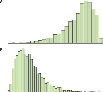
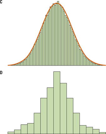
For Exercises 41–44, consider the accompanying distributions. What can we say about the values of the mean, median, and mode in relation to one another for the given histograms?
Question 3.41
41. The distribution in A
3.1.41
Mean < Median < Mode
Question 3.42
42. The distribution in B
Question 3.43
43. The distribution in C
3.1.43
Mean = Median = Mode
Question 3.44
44. The distribution in D
APPLYING THE CONCEPTS
Question 3.45
45. NFL Football, Southern Style. The table contains the population of all the teams in the National Football Conference South Division, along with the number of wins in the 2013 season.
- What is the population size, N, where the population is the NFC South Division?
- What is the population mean number of wins, μ?
| NFC South team | Wins |
|---|---|
| Carolina Panthers | 12 |
| New Orleans Saints | 11 |
| Atlanta Falcons | 4 |
| Tampa Bay Buccaneers | 4 |
3.1.45
(a) 4 (b) 7.75 wins
Question 3.46
46. New England Electoral Votes. The table contains the population of all the New England states, along with their electoral votes.
- What is the population size, N?
- Calculate the population mean number of electoral votes, μ.
| Electoral votes | |
|---|---|
| Connecticut | 7 |
| Maine | 4 |
| Massachusetts | 11 |
| New Hampshire | 4 |
| Rhode Island | 4 |
| Vermont | 3 |
Question 3.47
47. NFL Football, Southern Style. Refer to the population data in Exercise 45. Suppose we take a sample from the population, and we get the Carolina Panthers and the Atlanta Falcons.
- What is the sample size ?
- Calculate the sample mean number of wins, .
3.1.47
(a) 2 (b) 8 wins
Question 3.48
48. New England Electoral Votes. Refer to the population data in Exercise 46. Suppose we take a sample from the population, and get Massachusetts, Rhode Island, and Vermont.
- What is the sample size ?
- Calculate the sample mean number of electoral votes, .
Video Game Sales. The Chapter 1 Case Study looked at video game sales for the top 30 video games. The following table contains the total sales (in game units) and weeks on the top 30 list for a sample of five randomly selected video games. Use this information for Exercises 49 and 50.
| Video game | Total sales in millions of units |
Weeks |
|---|---|---|
| Super Mario Bros. U for WiiU | 1.7 | 78 |
| NBA 2K14 for PS4 | 0.6 | 27 |
| Battlefield 4 for PS3 | 0.9 | 29 |
| Titanfall for XBoxOne | 1.2 | 10 |
| Yoshi's New Island for 3DS | 0.2 | 10 |
Question 3.49
videogamereg
49. Find the following measures of center for total sales.
- Mean
- Median
3.1.49
(a) 0.92 million units (b) 0.9 million units
Question 3.50
videogamereg
50. Calculate the following measures of center for weeks.
- Mean
- Median
 Darts and the Dow Jones.
The following table contains a random sample of eight days from the Chapter 3 Case Study data set, indicating the stock market gain or loss for the portfolio chosen by the random darts, as well as the Dow Jones Industrial Average gain or loss for that day. Use this information for Exercises 51 and 52.
Question 3.51
51. Find the following measures of center for the darts stock returns.
- Mean
- Median
3.1.51
(a) 9.45 (b) 14.05
Question 3.52
dartsdjia
52. Find the following measures of center for the DJIA.
- Mean
- Median
| Darts | DJIA |
|---|---|
| −27.4 | −12.8 |
| 18.7 | 9.3 |
| 42.2 | 8 |
| −16.3 | −8.5 |
| 11.2 | 15.8 |
| 28.5 | 10.6 |
| 1.8 | 11.5 |
| 16.9 | −5.3 |
Age And Height. The following table provides a random sample from the Chapter 4 Case Study data set body_females, showing the age and height of the eight women. Use this information for Exercises 53 and 54.
| Age | Height |
|---|---|
| 40 | 63.5 |
| 28 | 63 |
| 25 | 64.4 |
| 34 | 63 |
| 26 | 63.8 |
| 21 | 68 |
| 19 | 61.8 |
| 24 | 69 |
Question 3.53
ageheight
53. Find the following measures of center for the women's ages.
- Mean
- Median
3.1.53
(a) 27.125 years (b) 25.5 years
Question 3.54
ageheight
54. Find the following measures of center for the women's heights.
- Mean
- Median
Saturated Fat and Calories. The table contains the calories and saturated fat in a sample of ten food items. Use this information for Exercises 55 and 56.
Question 3.55
satfatcorr
55. Find the following measures of center for calories.
- Mean
- Median
3.1.55
(a) 192.2 calories (b) 172 calories
Question 3.56
satfatcorr
56. Find the following measures of center for the grams of saturated fat.
- Mean
- Median
| Food item | Calories | Grams of saturated fat |
|---|---|---|
| Chocolate bar (1.45 ounces) | 216 | 7.0 |
| Meat & veggie pizza (large slice) |
364 | 5.6 |
| New England clam chowder (1 cup) |
149 | 1.9 |
| Baked chicken drumstick (no skin, medium size) |
75 | 0.6 |
| Curly fries, deep-fried (4 ounces) |
276 | 3.2 |
| Wheat bagel (large) | 375 | 0.3 |
| Chicken curry (1 cup) | 146 | 1.6 |
| Cake doughnut hole (one) | 59 | 0.5 |
| Rye bread (1 slice) | 67 | 0.2 |
| Raisin bran cereal (1 cup) | 195 | 0.3 |
Table 6 contains the trade balance currently maintained by the United States with a sample of 9 countries, for the month of June 2014. Use this data for Exercises 57–60.
| Country | Trade balance ($ billions) |
|---|---|
| Brazi | 1 |
| France | −1.2 |
| Germany | −5.6 |
| India | −1.3 |
| Italy | −2.4 |
| Japan | −5.6 |
| South Korea | −1.8 |
| Saudi Arabia | −1.8 |
| United Kingdom | 0 |
Question 3.57
57. Find the sample size, .
3.1.57
9
Question 3.58
58. Calculate the sample mean trade balance, .
Question 3.59
59. Find the median.
3.1.59
–$1.8 billion
Question 3.60
60. Find the modes.
Table 7 contains the number of cylinders, the engine size (in liters), the fuel economy (miles per gallon [mpg], city driving), and the country of manufacture for six 2011 automobiles. Use this information for Exercises 61–65.
| Vehicle | Cylinders | Engine size |
City mpg |
Country of manufacture |
|---|---|---|---|---|
| Cadillac CTS | 6 | 3.0 | 18 | USA |
| Ford Fusion Hybrid | 4 | 2.5 | 41 | USA |
| Ford Taurus | 6 | 3.5 | 18 | USA |
| Honda Civic | 4 | 1.8 | 25 | Japan |
| Rolls Royce | 12 | 6.7 | 11 | UK |
| Toyota Camry Hybrid |
4 | 2.4 | 31 | Japan |
Question 3.61
cylinderengine
61. Find the following for the number of cylinders:
- Mean
- Median
- Mode
3.1.61
(a) 6 cylinders (b) 5 cylinders (c) 4 cylinders
Question 3.62
cylinderengine
62. Refer to your work in Exercise 61. Which measure of center do you think is most representative of the typical number of cylinders? Explain.
Question 3.63
cylinderengine
63. Find the following for the engine size:
- Mean
- Median
- Mode
3.1.63
(a) 3.317 liters (b) 2.75 liters (c) No mode
Question 3.64
cylinderengine
64. Find the following for the city mpg:
- Mean
- Median
- Mode
Question 3.65
cylinderengine
65. Find the mode for country of manufacture.
3.1.65
USA
Use the information in Table 8 to answer Exercises 66–68, which gives the number of wins for the top 10 NASCAR racing drivers in various categories.
| Rank | Driver | Total | Super speedways |
Short tracks |
|---|---|---|---|---|
| 1 | Darrell Waltrip | 84 | 18 | 47 |
| 2 | Dale Earnhardt | 76 | 29 | 27 |
| 3 | Jeff Gordon | 75 | 15 | 15 |
| 4 | Cale Yarborough | 69 | 15 | 29 |
| 5 | Richard Petty | 60 | 19 | 23 |
| 6 | Bobby Allison | 55 | 24 | 12 |
| 7 | Rusty Wallace | 55 | 5 | 25 |
| 8 | David Pearson | 45 | 20 | 1 |
| 9 | Bill Elliott | 44 | 16 | 2 |
| 10 | Mark Martin | 35 | 5 | 7 |
Question 3.66
nascar
66. Refer to the super speedways data. Find the following:
- Mean
- Median
- Mode
Question 3.67
nascar
67. Refer to the short tracks data. Find the following:
- Mean
- Median
- Mode
3.1.67
(a) Mean = 18.8 (b) Median = 19 (c) No mode
Question 3.68
nascar
68. Refer to the totals data. Find the following:
- Mean
- Median
- Mode
For Exercises 69–73, refer to Table 9, which lists the top five mass market paperback fiction books for the week of July 1, 2014, as reported by the New York Times.
| Rank | Title | Author | Price |
|---|---|---|---|
| 1 | A Game of Thrones | George R. R. Martin | $7.83 |
| 2 | Takedown Twenty | Janet Evanovich | $7.64 |
| 3 | Inferno | Dan Brown | $8.48 |
| 4 | A Dance with Dragons | George R. R. Martin | $6.71 |
| 5 | The 9th Girl | Tami Hoag | $8.47 |
Question 3.69
69. Find the mean, median, and mode for the price of these five books on the best-seller list. Suppose a salesperson claimed that the price of a typical book on the best-seller list is less than $14. How would you use these statistics to respond to this claim?
3.1.69
$7.83, 7.83, no mode, A typical book on the best-sellers list would cost less than $14.00 since the mean and median are all less than $14.
Question 3.70
70. Linear transformations. Add $10 to the price of each book.
- Now find the mean of these new prices.
- How does this new mean relate to the original mean?
- Construct a rule to describe this situation in general.
Question 3.71
71. Linear transformations. Multiply the price of each book by 5.
- Now find the mean of these new prices.
- How does this new mean relate to the original mean?
- Construct a rule to describe this situation in general.
3.1.71
(a) $39.13 (b) The new mean is 5 times the original mean. (c) If each value of a data set is multiplied by a number , the mean of the resulting data set will be the mean of the original data set times .
Question 3.72
72. Find the mode for the following variables:
- Price
- Author
Question 3.73
73. Explain whether it makes sense to find the mean or median of the variable author.
3.1.73
It does not make sense to find the mean and the median of the variable author because the variable author is a categorical variable.
Mode of Categorical Data. The New York City Police Department tracks the number and type of traffic violations. The table contains a random sample of 12 traffic violations and the borough in which they occurred (Manhattan or Brooklyn). Use the data for Exercises 74–76.
| Violation type | Borough | Violation type | Borough |
|---|---|---|---|
| Cell phone | Brooklyn | Disobey sign | Manhattan |
| Safety belt | Manhattan | Speeding | Brooklyn |
| Cell phone | Brooklyn | Safety belt | Manhattan |
| Cell phone | Manhattan | Disobey sign | Manhattan |
| Speeding | Brooklyn | Disobey sign | Brooklyn |
| Safety belt | Manhattan | Cell phone | Manhattan |
Question 3.74
74. Find the mode for violation type. Does this mean that most violations are of this type?
Question 3.75
75. Calculate the mode for borough.
3.1.75
Manhattan
Question 3.76
76. Does the idea of the mean or median of these two variables make any sense? Explain clearly why not.
Car Model Years. The dotplot in Figure 9 represents the model year for a sample of cars in a used car lot. Refer to the dotplot for Exercises 77–79.
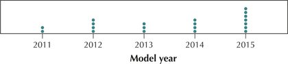
Question 3.77
77. What are the mean, median, and mode of the model year?
3.1.77
Mean = 2013.5, Median = 2014, Mode = 2015
Question 3.78
78. Calculate a new statistic “age of the car in 2015” as follows: take the model year and subtract it from 2015.
- Find the mode of the car ages.
- Find the mean and median of the car ages.
Question 3.79
79. What will be the mean, median, and mode of the car ages in 2025?
3.1.79
Mean = 11.5 years, Median = 11 years, Mode = 10 years
Question 3.80
80. Five friends have just had dinner at the local pizza joint. The total bill came to $30.60. What is the mean cost of each person's meal?
Question 3.81
81. Lindsay just bought four shirts at the boutique in the mall, costing a total of $84.28. What was the mean cost of each shirt?
3.1.81
$21.07
Dealing with Missing Data. Exercises 82–85 ask you to calculate measures of center when one of the values is missing.
Question 3.82
82. The mean cost of a sample of five items is $20. The cost of four of the items is as follows: $25, $15, $15, $20. What is the cost of the 5th item?
Question 3.83
83. The mean size of four downloaded music files is 3 Mb (megabytes). The size of three of the files is as follows: 5 Mb, 2 Mb, 3 Mb. What is the length of the 4th music file?
3.1.83
2 Mb
Question 3.84
84. The median number of students in a sample of seven statistics classes is 25. The ordered values are: 20, 22, 24, __, 27, 27, 28. What is the missing value?
Question 3.85
85. The median number of academic credits taken in a sample of six students is 15. The ordered values are: 12, 12, 14, __, 17, 17. What is the missing value?
3.1.85
16
Nutrition Ratings of Breakfast Cereals. Refer to the following information for Exercises 86–89. (Note that Minitab denotes both the sample size and the population size as .) The data represent the nutrition rate of 59 cereals based on sugar content, vitamin content, and so on.
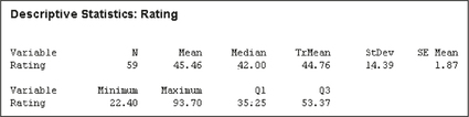
Question 3.86
86. Find the following sample statistics.
- The sample size
- The sample mean
- The sample median
- The highest and lowest ratings in the sample
Question 3.87
87. What do these statistics tell us about the skewness of the distribution?
3.1.87
The mean is larger than the median, which implies the distribution is positively skewed.
Question 3.88
88. Linear Transformations. If we take each cereal rating and subtract 5 from it, how would that affect the mean, median, and mode? Would it affect each of the measures equally?
Question 3.89
89. Linear Transformations. If we cut each of the cereals' ratings in half, how would that affect the mean, median, and mode? Would it affect each of the measures equally?
3.1.89
The mean, median and mode will all be halved. Each statistic will be affected equally.
BRINGING IT ALL TOGETHER
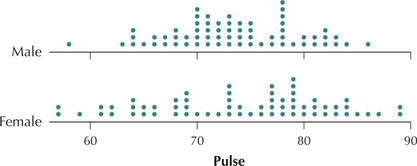
Pulse Rates for Men and Women. To answer Exercises 90–93, refer to Figure 10, which includes comparative dotplots of the pulse rates for males and females.2
Question 3.90
90. Examine Figure 10.
- Without doing any calculations, what is your impression of which gender, if any, has the higher overall pulse rate?
- Find the mean pulse rate for the males by estimating the location of the balance point.
- Find the mean pulse rate for the females by estimating the location of the balance point.
- Based on (b) and (c), which gender has the higher mean pulse rate? Does this agree with your earlier impression?
Question 3.91
91. Find the following medians:
- The median pulse rate for the males
- The median pulse rate for the females
- Which gender has the higher median pulse rate? Does this agree with your findings for the mean earlier?
3.1.91
(a) 73 (b) 76 (c) Females; yes
Question 3.92
92. Find the following modes:
- The mode pulse rate for the males
- The mode pulse rate for the females
- Which gender has the higher mode pulse rate? Does this agree with your findings for the mean earlier?
Question 3.93
 93. What if the fastest pulse rate for the men was a typo and should have been an unspecified lower pulse rate? Describe how and why this change would have affected the following, if at all. Would they increase, decrease, or remain unchanged? Or is there insufficient information to tell what would happen? Explain your answers.
- The mean men's pulse rate
- The median men's pulse rate
- The mode men's pulse rate
3.1.93
(a) Decrease (b) Unchanged (c) Unchanged
Question 3.94
statebusinesses
94. Trimmed Mean. Because the mean is sensitive to extreme values, the trimmed mean was developed as another measure of center. To find the 10% trimmed mean for a data set, omit the largest 10% of the data values and the smallest 10% of the data values, and calculate the mean of the remaining values. Because the most extreme values are omitted, the trimmed mean is less sensitive, or more robust (resistant), than the mean as a measure of center. For the data in the table, calculate the following:
- The mean
- The 10% trimmed mean
- The 20% trimmed mean
The data represent the number of business establishments in a sample of states.
| State | Businesses (1000s) |
State | Businesses (1000s) |
|---|---|---|---|
| Alabama | 3.8 | Michigan | 7.5 |
| Arizona | 7.9 | Minnesota | 6.1 |
| Colorado | 8.9 | Missouri | 5.9 |
| Connecticut | 3.1 | Ohio | 9.5 |
| Georgia | 10.3 | Oklahoma | 3.8 |
| Illinois | 11.9 | Oregon | 5.4 |
| Indiana | 5.6 | South Carolina | 4.6 |
| Iowa | 2.7 | Tennessee | 5.4 |
| Maryland | 5.7 | Virginia | 8.6 |
| Massachusetts | 6.3 | Washington | 9.3 |
Question 3.95
95. Challenge Exercise. In general, would you expect the trimmed mean to be larger, smaller, or about the same as the mean for data sets with the following shapes?
- Right-skewed data
- Left-skewed data
- Symmetric data
3.1.95
(a) Smaller (b) Larger (c) Same
Question 3.96
96. Midrange. Another measure of center is the midrange.
Because the midrange is based on the maximum and minimum values in the data set, it is not a robust statistic, but it is sensitive to extreme values. Calculate the midrange for the following data:
Question 3.97
97. Harmonic Mean. The harmonic mean is a measure of center most appropriately used when dealing with rates, such as miles per hour (mph). The harmonic mean is calculated as
where is the sample size and the 's represent rates, such as the speeds in mph. Emily walked five miles today, but her walking speed slowed as she walked farther. Her walking speed was 5 mph for the first mile, 4 mph for the second mile, 3 mph for the third mile, 2 mph for the fourth mile, and 1 mph for the fifth mile. Calculate her harmonic mean walking speed over the entire five miles.
3.1.97
2.190 mph
Question 3.98
98. Challenge Exercise. The (arithmetic) mean for Emily's five-mile walk in Exercise 97 is 3 mph. Explain clearly why the value you calculated for the harmonic mean in Exercise 97 makes more sense than this arithmetic mean of 3 mph. (Hint: Consider time.)
Question 3.99
99. Geometric Mean. The geometric mean is a measure of center used to calculate growth rates. Suppose that we have positive values; then the geometric mean is the th root of the product of the values. Jamal has been saving money in an account that has had 4% growth, 6% growth, and 10% growth over the last three years. Calculate the average growth rate over these three years. (Hint: Find the geometric mean of 1.04, 1.06, and 1.10 and subtract 1.)
3.1.99
Geometric mean = 1.0664, 6.64% growth
CONSTRUCT YOUR OWN DATA SETS
Question 3.100
100. Construct your own data set with , where the mean, the median, and the mode are all the same. Yes, just make up your own list of numbers, as long as the mean, median, and mode are all the same. Draw a dotplot. Comment on the skewness of the distribution.
Question 3.101
101. Construct your own data set with , where the mean is greater than the median, which is greater than the mode. Draw a dotplot. Comment on the skewness of the distribution.
3.1.101
Answers will vary.
Question 3.102
102. Construct your own data set with , where the mode is greater than the median, which is greater than the mean. Draw a dotplot. Comment on the skewness of the distribution.
Question 3.103
103. Construct your own data set with . Let the mean and median be equal. Now, alter the three data values so that the mean of the altered data set has increased, while the median of the altered data set has decreased.
3.1.103
Answers will vary.
![]() Use the Mean and Median applet for Exercises 104 and 105.
Use the Mean and Median applet for Exercises 104 and 105.
Question 3.104
104. Insert three points on the line by clicking just below it: two near the left side and one near the middle.
- Click and drag the rightmost point to the right.
- Describe what happens to the mean when you do this.
- Describe what happens to the median when you do this.
Question 3.105
105. Explain why each of the measures behaves the way it does in the previous exercise.
3.1.105
Answers will vary.
WORKING WITH LARGE DATA SETS
Open the VideoGameSales data set from the Chapter 1 Case Study. The data set represents a sample. Use technology to do the following.  videogamesales
Question 3.106
videogamesales
106. Find the mean and median weekly sales.
Question 3.107
videogamesales
107. Suppose we remove the biggest seller for the week, Minecraft for PS3, from the data. Given what you have learned about the sensitivity of the mean to the presence of extreme values, which measure do you expect will change the most, the mean or the median?
Question 3.108
videogamesales
108. Recalculate the mean and the median of weekly sales, this time omitting Minecraft for PS3. Was your intuition in Exercise 107 confirmed?
Question 3.109
videogamesales
109. Compute the mean and median total sales for the 30 games.
Question 3.110
videogamesales
110. Identify the video game with the largest total sales. Omit this video game, and recompute the mean and median total sales. Which measure of center was more sensitive to the removal of the extreme value?
Question 3.111
videogamesales
111. Find the mode for each of the following variables:
- Platform
- Studio
- Game type
Question 3.112
videogamesales
112. Compute the mean, median, and mode for the variable weeks on list.
Question 3.113
videogamesales
113. What if we add a certain unknown amount to each value in the variable weeks on list? Describe what will happen to the following measures of center.
- Mean
- Median
- Mode