5.1 Introducing Probability
 This page includes Statistical Videos
OBJECTIVES By the end of this section, I will be able to …
- Understand the meaning of an experiment, an outcome, an event, and a sample space.
- Describe the classical method of assigning probability.
- Explain the Law of Large Numbers and the relative frequency method of assigning probability.
Imagine you are striding down the midway of your local town fair, when a particular game of chance catches your eye. The object of this game is to roll a six on a single roll of a single fair die. If you do so, you win $5. It costs $1 to play the game. What is the likelihood of winning?
To show how to solve this problem, we must first introduce the building blocks of probability.
1 Building Blocks of Probability
Our daily lives are filled with uncertainty, seemingly governed by chance. We try to cope with uncertainty by estimating the chances that a particular event will occur. We are expected, on a daily basis, to make intelligent decisions about probabilities. Consider the following scenarios, and think about how the italicized words all refer to uncertainty:
- What is the chance that there will be a speed trap on this stretch of I-95 on a particular day?
- What is the likelihood that this lottery ticket will make me rich?
- What is the probability that this throw of the dice will come up a seven?
Sometimes, the amount of uncertainty in our daily lives is so great that there appears to be no order to the world whatsoever. However, if you look closely, there are patterns in randomness. In this chapter, we learn to become better decision makers by becoming acquainted with the tools of probability in order to quantify many of the uncertainties of everyday life.
The probability of an outcome represents the chance or likelihood that the outcome will occur.
Let us acquaint ourselves with the building blocks of probability, starting with the concept of an experiment. In probability, an experiment is any activity for which the outcome is uncertain. Consider the stock market, for example. Suppose you own 100 shares of Consolidated Widgets and are interested in what the share price will be at the end of trading tomorrow. Will the share price increase or decrease? The actual result is uncertain, so this is an example of an experiment. Each of the possible results of the experiment is called an outcome. Another example of an experiment is when you toss a coin. In the coin-toss experiment, the result may be heads or it may be tails. The collection of all possible outcomes is called the sample space. The sample space for the coin-toss experiment is {heads, tails} or {H, T}. Following are some common experiments, together with their sample spaces.
We use brackets like these { } to enclose a set of outcomes.
| Experiment | Sample space |
|---|---|
| Roll a single six-sided die | {1, 2, 3, 4, 5, 6} |
| Toss two coins | {HH, HT, TH, TT} |
| Play a video game | {win, lose} |
We use the building blocks of probability to investigate the likelihood of an outcome or event.
Building Blocks of Probability
An experiment is any activity for which the outcome is uncertain.
An outcome is the result of a single performance of an experiment.
The collection of all possible outcomes is called the sample space. We denote the sample space S.
An event is a collection of outcomes from the sample space. To find the probability of an event, add up the probabilities of all the outcomes in the event.
The following table shows some typical events for the experiments in the table on page 240.
| Experiment | Sample space | Typical events |
|---|---|---|
| Roll a single die | {1, 2, 3, 4, 5, 6} |
E:roll an even number={2,4,6} L:roll a 4 or larger={4,5,6} |
| Toss two coins | {HH, HT, TH, TT} |
H:exactly one head ={HT,TH} T:at most one tail ={HH,HT,TH} |
| Play a video game | {win, lose} |
W:win ={win} L:lose ={lose} |
When we talk about the probability of some outcome, we are referring to a number that indicates how likely the particular outcome is. The notation P(A) stands for “the probability that outcome A occurred.” Say we define outcome W to be “you win the video game.” Then “the probability that you win the video game” can be denoted as P(W). Probabilities abide by the following rules.
Rules of Probability
- The probability P(E) for any event E is always between 0 and 1, inclusive. That is, O≤P(E)≤1.
- Law of Total Probability: For any experiment, the sum of all the outcome probabilities in the sample space must equal 1.
Developing Your Statistical Sense
A Different Perspective
As you read this chapter, notice that the perspective differs from that in previous chapters. Earlier, we were looking at a data set and trying to describe it graphically and numerically. Now, instead of trying to describe a data set, we are faced with an experimental situation, and our task is to calculate probabilities associated with various outcomes in the experiment.
 If the probability that you calculated is negative or greater than 1, then you should try again.
From the definition, the probability of an event is a proportion. Therefore, probability cannot be negative because proportions cannot be negative, and probability cannot be greater than 1 (100%) because an event cannot occur more than 100% of the time. A probability model is a table or listing of all the possible outcomes of an experiment, together with the probability of each outcome. A probability model must follow the Rules of Probability.
EXAMPLE 1 Probability models
For the following three scenarios, determine whether or not a valid probability model exists:
- You ask your friend what his favorite ice cream flavor is.
Outcome Probability Mint chocolate chip 0.25 Pistachio −0.25 Vanilla 0.50 Other 0.50 - You ask another friend to go to a concert.
Outcome Probability Yes 0.5 No 0.5 Maybe 0.5 - You play a single game of roulette and bet on red.
Outcome Probability Win 0.47 Lose 0.53
Solution
To be a valid probability model, each scenario must meet both rules of probability.
- The probability that your friend likes pistachio ice cream may not be very high, but it cannot be negative. This violates the first rule of probability that every event must have probability between zero and one. Note that, even though the second rule of probability is fulfilled (the probabilities sum to one), we nevertheless do not have a valid probability model here.
- Here, the first rule of probability is met, but the second one is violated. The sum of the three probabilities is 0.5+0.5+0.5=1.5. This is not equal to one, so that we do not have a valid probability model here either.
- Here, both probabilities lie between zero and one, so that the first rule of probability is met. Also, the sum of the two probabilities is 0.47+0.53=1.00, which fulfills the second rule of probability. Therefore, (c) represents a valid probability model.
NOW YOU CAN DO
Exercises 11–16.
Throughout the remainder of this book, you will often be asked to calculate the probability of various events. Table 1 contains the meanings of some values of probability.
| Probability value | Meaning |
|---|---|
| Near 0 | Outcome or event is very unlikely. |
| Equal to 0 | Outcome or event cannot occur. |
| Near 1 | Outcome or event is nearly certain to occur. |
| Equal to 1 | Outcome or event is certain to occur. It's “a sure thing.” |
| Low | Outcome or event is unusual, say, with probability less than 0.05. |
| High | Outcome or event is likely to happen. |
The threshold of an unusual event depends on the specific experiment; the 0.05 probability for an unusual event is not set in stone.
Higher probability values are associated with higher likelihood of occurrence. An outcome with probability 0.5 will happen about half of the time. An outcome with probability 0.95 is very likely. We say that an outcome or event is unusual if its probability is below a certain threshold, say, 0.05.
EXAMPLE 2 Determining unusual or likely outcomes
For the following probabilities, determine the meaning of the indicated probability:
- The weatherman said that the chance of rain tonight was near 100%.
- The coach said that after that last loss, the team had no chance to make the playoffs.
- The doctor said that the chance of a negative reaction to the planned procedure was 3%.
Solution
- A value of near 100% is near 1. Therefore, it is nearly certain to occur that we will have rain tonight.
- No chance means a probability equal to zero. Therefore, it cannot occur that the team will make the playoffs.
- The chance of a negative reaction is 3%, or 0.03. This probability is low (for example, below a certain threshold, such as 0.05), so we conclude that it would be unusual for a negative reaction to the planned procedure to occur.
NOW YOU CAN DO
Exercises 17–20.
YOUR TURN#1
For the following probabilities, determine the meaning of the indicated probability:
- The stockbroker said that the chance for a recession was near zero.
- The salesperson said that your chance of satisfaction with the purchase of a new car was 100%.
(The solutions are shown in Appendix A.)
When we perform an experiment, it is a “sure thing” that one of the outcomes in the sample space will occur. For example, when you toss a coin, you know that it will be either heads or tails. Put into probability terms, the sum of the probabilities of all the individual outcomes must equal 1, which is the Law of Total Probability we mentioned above.
2 Classical Method of Assigning Probability
Many people have a certain degree of intuition when it comes to assigning probabilities. For example, when asked what the chances are of rolling a 6 on a single toss of a fair die, many people would quite correctly answer 1/6. However, intuition can often let us down. For example, when asked what the chances are of observing two heads when you toss a fair coin twice, many people would incorrectly respond 1/3. (“Well, it’s either both heads or both tails or one of each.” The correct answer is in fact 1/4.) In this section, we learn how to quantify our methods of assigning probabilities, so that we don’t have to depend on intuition alone.
Three methods for assigning probabilities are available:
- Classical method
- Relative frequency method
- Subjective method
We first take a close look at the classical method. Later in this section, we will examine the relative frequency method and the subjective method.
Many experiments are structured so that each experimental outcome is equally likely. Equally likely outcomes are outcomes that have the same probability of occurring. For example, if you toss a fair coin, the probability of observing either of the outcomes—heads or tails—is the same. The classical method of assigning probabilities is used when an experiment has equally likely outcomes.
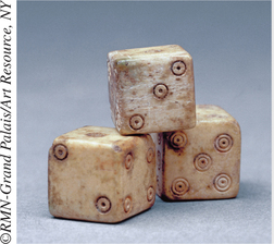
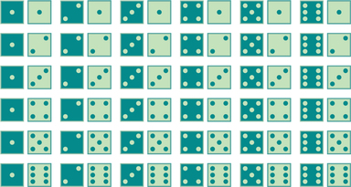
Did you know? People have been tossing dice for a long time. Archaeologists have dug up dice from Roman ruins looking just the same as ours. These three dice were uncovered from the ruins of Pompeii buried by the eruption of Mount Vesuvius in the first century A.D.
Classical Method of Assigning Probabilities
Let N(E) and N(S) denote the number of outcomes in event E and the sample space S, respectively. If the experiment has equally likely outcomes, then the probability of event E is
P(E)=number of outcomes in Enumber of outcomes in sample space=N(E)N(S)
EXAMPLE 3 Classical method: Single draw from a deck of cards
Find the probability of drawing an ace when drawing a single card at random from a deck of cards.
Solution
The sample space for the experiment in which a subject chooses a single card at random from a deck of cards is given in Figure 1. If the card is chosen truly at random, then it is reasonable to assume that each card has the same chance of being drawn. Each card is equally likely to be drawn, so we can use the classical method to assign probabilities.
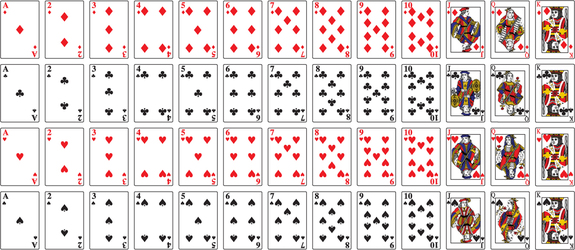
A total of 52 outcomes are included in this sample space, so N(S)=52. Let E be the event that an ace is drawn. Event E consists of the four aces {A ♥, A♦, A♣, A♠}, so N(E)=4. Therefore, the probability of drawing an ace is
P(E)=N(E)N(S)=452=113
NOW YOU CAN DO
Exercises 21–24.
YOUR TURN#2
Find the probability of the following events when drawing a single card at random from a deck of cards:
- a heart
- a black card
(The solutions are shown in Appendix A.)
EXAMPLE 4 Classical method: Single fair die
Recall the town fair example (page 240). In the game, you win if you roll a 6 on a single roll of a single fair die. Find the probability of winning the game.
Solution
The sample space for a single die toss consists of six outcomes, {1,2,3,4,5,6}. When the six outcomes are equally likely, we say that the die is fair. If the outcomes are not equally likely, then the die is loaded or defective. If we assume the die is fair, then, because the sum of the probabilities of the n=6 outcomes must equal 1, the probability of any particular outcome must equal 1/6, using the classical method. We write
probability of winning = P(W)=1/6
NOW YOU CAN DO
Exercises 25–30.
YOUR TURN#3
For the experiment in Example 4, find the following probabilities:
- Not winning the game
- Rolling a 5
(The solutions are shown in Appendix A.)
Tree Diagrams
A tree diagram is a graphical display that allows us to list all the outcomes in the sample space of a multistage experiment. The next example shows how to construct a tree diagram.
EXAMPLE 5 List all outcomes in a sample space using a tree diagram
Suppose our experiment is to toss a fair coin twice.
- Construct a tree diagram.
- Use the tree diagram to list all the outcomes in the sample space.
Solution
- Think of this experiment as a two-stage process:
- Stage 1: Toss the coin the first time.
Stage 2: Toss the coin the second time.
Page 246Figure 2 shows the tree diagram for the experiment of tossing a fair coin twice. Note the branches for Stage 1: the first time the coin is tossed, it can come up heads or tails. At Stage 2, the tree diagram again has branches for either heads or tails.
- The sample space for the experiment of tossing a coin twice is {HH, HT, TH, TT}. There are N(S)=4 outcomes in the sample space.
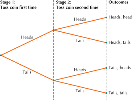 FIGURE 2 Tree diagram for the experiment of tossing a fair coin twice.
NOW YOU CAN DO
Exercises 31–38.
YOUR TURN#4
Suppose our experiment is to toss a fair coin three times.
- Construct a tree diagram.
- Use the tree diagram to list all the outcomes in the sample space.
(The solutions are shown in Appendix A.)
Note that two possible outcomes can occur at Stage 1 of this two-stage experiment and two possible outcomes when flipping the coin at Stage 2. To determine the number of outcomes in the entire experiment, the counting rule is simply to multiply the number of possible outcomes at each stage. In this two-stage experiment, 2×2=4 possible outcomes, which is the number of outcomes we see in the sample space.
EXAMPLE 6 Classical method: Tossing a fair coin twice
Find the probability of obtaining one heads and one tails when a fair coin is tossed twice.
Solution
It is reasonable to assume that the N(S)=4 outcomes in the sample space {HH, HT, TH, TT} are equally likely. The coin doesn’t remember what occurred at Stage 1, so the probabilities at Stage 2 are precisely the same as at Stage 1. Also, recall from the Law of Total Probability that the sum of the probabilities of all the outcomes in the sample space must equal 1. Thus, each of the four outcomes must have probability 1/4. Let E be the event that one heads and one tails is obtained. Then E={HT,TH}, so N(E)=2. Thus,
P(E)=number of outcomes in Enumber of outcomes in sample space=N(E)N(S)=24=12
NOW YOU CAN DO
Exercises 39–42.
YOUR TURN#5
For the experiment in Example 6, find the following probabilities:
- Two heads
- Two tails
(The solutions are shown in Appendix A.)
EXAMPLE 7 Finding probabilities for the experiment of tossing two fair dice
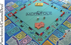
Imagine that you are playing Monopoly with your dormitory roommate, and the loser has to do the laundry for both of you for the rest of the semester. You have a hotel on Boardwalk, and if your roommate lands on it, you will surely win. Right now your roommate’s piece is on Short Line: if he or she rolls a 4, you will win and get your laundry done free for the remainder of the semester. Put into statistical terms, the experiment is to toss two fair dice and observe the sum of the two dice. Find the probability of rolling a sum of 4 when tossing two fair dice.
Solution
It is reasonable to assume that each of these N(S)=36 outcomes in the sample space (Figure 3) is equally likely. The experiment of tossing two dice can be viewed as a two-stage experiment, where we add the result from the first die to the result from the second die. If a 5 appears on the first (say, dark green) die, and a 3 appears on the second (light green) die, the overall outcome is (5,3), with the resulting sum equal to 8. Note that the outcome (5,3) is not the same as the outcome (3,5), where the dark green die comes up 3 and the light green die comes up 5.
Let E denote the event that your roommate rolls a sum equal to 4. Then the outcomes that belong in this event are E:{(3,1)(2,2)(1,3)}, so N(E)=3. The outcomes are equally likely, so we can use the classical method for finding probabilities of events.
P(E)=number of outcomes in Enumber of outcomes in sample space=N(E)N(S)=336=112
The probability that your roommate will land on Boardwalk on this throw of the dice is 1/12.
NOW YOU CAN DO
Exercises 43–50.
YOUR TURN#6
For the experiment in Example 7, find the following probabilities:
- Rolling a sum of 7 with the two dice
- Rolling boxcars (sum of 12 with the two dice)
- Rolling snake eyes (sum of 2 with the two dice)
(The solutions are shown in Appendix A.)
EXAMPLE 8 Inappropriate use of the classical method
Watch a lot of YouTube? Hate the in-stream ads? According to Social Strand Media, 75% of in-stream ads are skippable (www.slideshare.net/SocialStrand/social-media-stats-2014). Suppose we choose one in-stream ad at random. Define the following events:
- C:The randomly chosen in-stream ad is skippable.
- D:The randomly chosen in-stream ad is not skippable.
Determine whether the classical method can be used to assign probability to events C and D.
Solution
Because more than half of in-stream ads are skippable, if we choose one at random, we are more likely to find a skippable one than a non-skippable one. Therefore, the events C and D are not equally likely. It would be inappropriate to use the classical method of assigning probabilities for this experiment because the classical method can be used only when all the outcomes of an experiment are equally likely.
The proper method for solving this problem is the relative frequency method, which we discuss next.
3 Relative Frequency Method
In Example 4, we need the classical method to find that the probability of rolling a 6 with a fair die is 1/6. What does this probability mean? Remember that the definition of probability included the phrase “long-term proportion.” The next example demonstrates what we mean by “long-term.”
EXAMPLE 9 Simulating the long-term proportion of 6s in a fair die roll
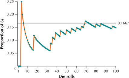
Suppose we want to investigate the proportion of 6s we observe if we roll a fair die 100 times. We can use technology, such as the TI-83/84 used here, to help us simulate rolling a fair die a large number of times. A simulation uses methods such as rolling dice or computer generation of random numbers to generate results from an experiment. The actual die rolls from our simulation are shown here, in order, with the 6s in boldface.
| 1 4 4 6 2 4 3 2 1 3 4 3 3 4 3 3 6 3 5 5 1 5 3 5 5 2 1 3 1 1 1 5 5 6 3 6 2 1 6 5 5 4 4 6 5 4 1 1 4 6 |
| 4 2 2 2 6 3 2 5 5 6 1 1 3 1 6 5 4 6 6 5 5 5 2 5 5 3 4 2 4 6 4 5 5 1 6 3 1 1 1 3 5 4 2 3 3 3 6 2 5 3 |
Thus, the first die roll was a 1, so the proportion of 6s was 0/1. The second and third die rolls were 4s, so the proportion of 6s after 3 rolls was 0/3. On the fourth roll, a 6 appeared, so the proportion of 6s after the fourth roll was 1/4. Figure 4 provides a graph of the proportion of 6s in this simulation as the number of die rolls increased. Note that as the number of die rolls increases, the proportion of 6s tends to get closer to the horizontal line: 0.1667≈1/6.
The simulation was rerun—this time with 1000 die rolls. The resulting graph of the proportion of 6s is provided in Figure 5. Note that as the number of die rolls increases, the proportion of 6s approaches the line 0.1667≈1/6, and the fit is tighter with 1000 die rolls than with 100. This is what we mean by “long-term proportion.”
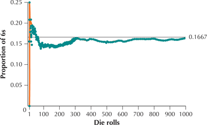
This example leads directly to the following law.
Law of Large Numbers
As the number of times that an experiment is repeated increases, the relative frequency (proportion) of a particular outcome tends to approach the probability of the outcome.
- For quantitative data, as the number of times that an experiment is repeated increases, the mean of the outcomes tends to approach the population mean.
- For categorical (qualitative) data, as the number of times that an experiment is repeated increases, the proportion of times a particular outcome occurs tends to approach the population proportion.
![]() The Law of Large Numbers for Proportions applet allows you to simulate coin tossing and observe the proportion of heads as the number of tosses increases.
The Law of Large Numbers for Proportions applet allows you to simulate coin tossing and observe the proportion of heads as the number of tosses increases.
Note: The relative frequency method may be used when previous information is available about the relative frequency of an event.
Relative Frequency Method
If we can't use the classical method for assigning probabilities, then the Law of Large Numbers gives us a hint about how we can estimate the probability of an event. It often happens that previous information is available about the relative frequency of an event. Relative frequency information can be used to estimate the probability of the event.
Note: Tree diagrams can be used for the relative frequency method as well as the classical method of assigning probability.
Relative Frequency Method of Assigning Probabilities
The probability of event E is approximately equal to the relative frequency of event E. That is,
P(E)≈relative frequency of E=frequency of Enumber of trials of experiment
The relative frequency method is also known as the empirical method.
EXAMPLE 10 Relative frequency method
 The Gardasil vaccine
The Case Study data set Gardasil provides the following relative frequency distribution for the variable Completed, indicating whether or not the patient completed the course of three Gardasil vaccinations. Use the relative frequency method to find the probability that a randomly chosen patient completed the treatment.
| Completed | Frequency | Relative frequency |
|---|---|---|
| Yes | 469 | 0.3319 |
| No | 944 | 0.6681 |
| Total | 1413 | 1.0000 |
Solution
Define the event.
C: Patient completed treatment.
We use the relative frequency method to find the probability of event C:
P(C)≈relative frequency of C=frequency of Cnumber of trials in experiment=4691413≈0.3319
NOW YOU CAN DO
Exercises 51–60.
YOUR TURN#7
Using the experiment from Example 10, do the following:
- Use a capital letter to define the event that a patient did not complete the treatment.
- Find the relative frequency of your event from (a).
- Assign your relative frequency from (b) as the probability that a patient did not complete the treatment.
(The solutions are shown in Appendix A.)
We can also use the relative frequency method to build a probability model with data that have been summarized in a table.
EXAMPLE 11 Probability models based on frequency tables
Table 2 contains the employment type for a sample of 1000 employed citizens of Fairfax County, Virginia.3 Use the data to construct the probability model by generating the relative frequencies and using the relative frequencies to estimate the probabilities for each employment type.
| Employment type | Count |
|---|---|
| Private company | 597 |
| Federal government | 141 |
| Self-employed | 97 |
| Private nonprofit | 92 |
| Local government | 59 |
| State government | 12 |
| Other | 2 |
Solution
We calculate the relative frequencies of each employment group by dividing the count (frequency) for each group by the sample size 1000. For example, the relative frequency for “Private Company” is 5971000=0.597. The relative frequency is then used to estimate the probability of selecting citizens who work at private companies in Fairfax County, Virginia. Filling in the remaining calculations produces the probability model in Table 3. Note that the table follows the Rules of Probability in that (a) each outcome has probability between 0 and 1, and (b) the sum of the probabilities of all the outcomes equals 1.0.
| Employment type | Probability |
|---|---|
| Private company | 0.597 |
| Federal government | 0.141 |
| Self-employed | 0.097 |
| Private nonprofit | 0.092 |
| Local government | 0.059 |
| State government | 0.012 |
| Other | 0.002 |
fairfaxemploy
NOW YOU CAN DO
Exercises 61 and 62.
EXAMPLE 12 Random draws using a probability model
Suppose we consider the probabilities in Table 3 as population values. Use technology to simulate random draws using the probability model in Table 3.
Solution
Using the Step-by-Step Technology Guide on page 252, we drew samples of sizes 10, 100, 1,000, and 10,000 from the probability model in Table 3. The results are shown in Table 4.
| Employment type | Rel freq n=10 |
Rel freq n=100 |
Rel freq n=1,000 |
Rel freq n=10,000 |
|---|---|---|---|---|
| Private company | 0.60 | 0.62 | 0.566 | 0.596 |
| Federal government | 0.20 | 0.15 | 0.15 | 0.143 |
| Self-employed | 0.10 | 0.11 | 0.109 | 0.991 |
| Private nonprofit | 0.10 | 0.07 | 0.106 | 0.914 |
| Local government | 0.00 | 0.04 | 0.055 | 0.056 |
| State government | 0.00 | 0.01 | 0.012 | 0.012 |
| Other | 0.00 | 0.00 | 0.002 | 0.002 |
Note that each relative frequency tends to approach its respective probability as the sample sizes grow larger.
Subjective method for assigning probability
Some cases have outcomes that are not equally likely (so the classical method does not apply) and there has been no previous research (so the relative frequency approach does not apply). For example, what is the probability that the Dow Jones Industrial Average will decrease today? In cases like this, there is no absolutely correct probability. Reasonable people can disagree reasonably over these probabilities. The idea is to consider all available information, tempered by our experience and intuition, and then assign a probability value that expresses our estimate of the likelihood that the outcome will occur. Finally, it should be noted that the subjective method should be used when the event is not (even theoretically) repeatable.
Subjective probability refers to the assignment of a probability value to an outcome based on personal judgment.
EXAMPLE 13 Subjective method for assigning probability
A financial analyst is interested in the probability that the Dow Jones Industrial Average will go down today. Suppose the Chairman of the Federal Reserve warned against inflation in a major speech yesterday. How would the financial analyst use this information to subjectively assign the probability that the stock market will go down today?
Solution
Through long professional experience, the financial analyst has seen the Dow go down—often, the day after speeches by the Federal Reserve Chairman warning against inflation. She therefore assigns a subjective probability that the probability the Dow Jones Industrial Average will go down today is 75%. Although the exact subjective probability assigned by other financial analysts may differ somewhat, most will probably share the opinion that the Dow will decrease today.