5 Probability

5.3 Conditional Probability

OBJECTIVES By the end of this section, I will be able to …

Calculate conditional probabilities.
Explain independent and dependent events.
Solve problems using the Multiplication Rule and recognize the difference between sampling with replacement and sampling without replacement.
Approximate probabilities for dependent events.
Apply Bayes' Rule to solve probability problems.

1 Introduction to Conditional Probability

As we progress through this book, you will notice a recurring theme: the more information available, the better. Very often, when we are investigating the probability of a certain event $A$ , we learn that another event $B$ has occurred. If events $A$ and $B$ are related, then the occurrence of event $B$ often influences the probability that event $A$ will occur.

Page 271

EXAMPLE 18 Having more information often affects the probability of an event

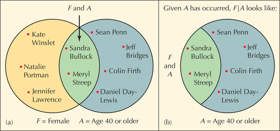
Table 19 contains the Academy Award winners for Best Actress and Best Actor for 2009–2014, along with their ages at the time of the award.

Table 5.52: Table 19 Oscar-winning actresses and actors, and their ages

Year	Best actress	Film	Age	Best actor	Film	Age
2009	Kate Winslet	The Reader	33	Sean Penn	Milk	48
2010	Sandra Bullock	The Blind Side	45	Jeff Bridges	Crazy Heart	60
2011	Natalie Portman	Black Swan	29	Colin Firth	The King's Speech	50
2012	Meryl Streep	Iron Lady	62	Jean Dujardin	The Artist	39
2013	Jennifer Lawrence	Silver Linings Playbook	22	Daniel Day- Lewis	Lincoln	55

Table 5.52: Source: www.oscars.org.

Table 20 is a contingency table, summarizing the information in Table 19, providing the counts of the performers' genders and whether the performer was under age 40.

Table 5.53: Table 20 Contingency table of Oscar-winning performers

	Female	Male	Total
Under age 40	3	1	4
Age 40 or older	2	4	6
Total	5	5	10

Now, if we choose a performer at random from Table 20, the probability of choosing a female is $P (F) = \frac{5}{10} = 0.5$ . But what if we were given the extra information that the performer is age 40 or older? How does this extra information affect the probability of selecting a female?

Solution

Notice that when we are given that the person is age 40 or older, we may restrict our attention to the performers who are age 40 or older in Table 20 (highlighted). In other words, this extra information reduces the number of possible outcomes in the sample space from the 10 performers to the 6 performers who are age 40 or older. Of these six performers, two of them are female. Thus, the probability of selecting a female, given that the performer is age 40 or older, is $2 / 6 = 1 / 3 \approx 0.33$ . The extra information we were given changed the probability of selecting a female, from $1 / 2$ to $1 / 3$ .

The extra information about a related event changed the probability of the event of interest. This type of probability is an example of what is called conditional probability.

Note: The vertical line | is read as the word “given.” Whatever follows the word “given” is assumed to have occurred already.

For two related events $A$ and $B$ , the probability of $B$ given $A$ is called a conditional probability and is denoted as $P (B | A)$ , or $P (B given A)$ .

Page 272

Thus, if we let $F$ represent the event that a female is selected and $A$ represent the event that the performer is age 40 or older, then

$P (F) = \frac{5}{10} = \frac{1}{2} but P (F given A) = P (F | A) = \frac{2}{6} = \frac{1}{3}$

Figure 17 can help us visualize how conditional probability works. The idea is that, once event A has occurred, the only chance for event $F$ to occur is in the overlap—the intersection $(F and A)$ . Therefore, the conditional probability that $F$ will occur, given that event $A$ has already taken place, is found by taking the ratio $P (F and A) / P (A)$ .

FIGURE 17 How conditional probability works.

Developing Your Statistical Sense

The difference between $P (F given A) and P (F and A)$

Students sometimes confuse the meanings of $P (F given A) with P (F and A)$ . The two are very different.

For $P (F and A)$ , neither $A$ nor $F$ has occurred. We don’t know if either will or will not occur. Instead, we need to determine the probability that events $F$ and $A$ both occurred. Look at Figure 17a. For finding $P (F and A)$ , we don’t know if our randomly chosen performer is female or is age 40 or older. Two of our 10 performers are both female and age 40 or older: Sandra Bullock and Meryl Streep. Thus, $P (F and A) = 2 / 10 = 1 / 5$ .
For $P (F given A) = P (F | A)$ , we assume that the event A has already occurred and now need to find the probability of event $F$ , given event $A$ . There is no probability involved with the event $A$ , because it has already occurred. Look at Figure 17b. For $P (F given A) = P (F | A)$ , we are given that the performer is age 40 or older; we know this event occurred. Therefore, we can restrict our attention solely to performers age 40 or older (event $A$ ). Of the six performers age 40 or older, two are female. Thus, $P (F given A) = P (F | A) = 2 / 6 = 1 / 3$ .

In general, the formula for computing conditional probability is given as follows.

Calculating Conditional Probability

The conditional probability that $B$ will occur, given that event $A$ has already taken place, equals

$P (B given A) = P (B | A) = \frac{P (A a n d B)}{P (A)} = \frac{N (A a n d B)}{N (A)}$

Page 273

EXAMPLE 19 Calculating conditional probability

Marketing companies are looking to statistical analysis and data mining in an effort to increase the customer response to their promotions. Therefore, these marketing companies are looking to hire more statistics-savvy students. Table 21 is adapted from a study on direct mail marketing. It contains the numbers of custom-ers who either responded or did not respond to a direct mail marketing campaign, along with whether they had a credit card on file with the company. The two events are:

$R : Responded to direct mail marketing campaign$
$C : Has a credit card on file$

Table 5.54: Table 21 Credit card status and marketing response

Response	Credit card on file?
Response	No	Yes	Total
Did not respond	161	79	240
Did respond	17	31	48
Total	178	110	288

Table 5.54: Source: Data Mining and Predictive Analytics, by Daniel Larose and Chantal Larose, Wiley Interscience, 2015.

Find the probability that a randomly chosen customer responded to the marketing campaign.
Calculate the probability that a randomly chosen customer both responded to the marketing campaign and has a credit card on file.
Find the conditional probability that a randomly selected customer responded, given that the customer has a credit card on file.

Solution

$P (R) = \frac{N (R)}{N (S)}$ . There are $N (R) = 48$ customers who did respond, and there are $N (S) = 288$ customers in this experiment. Thus,
$P (R) = \frac{N (R)}{N (S)} = \frac{48}{288} \approx 0.1667$
Here, we are looking for $P (R and C)$ , which is the intersection between $R$ and $C$ . Earlier, we learned that this is represented by the cell at the intersection of the “Did respond” row and the “Credit card yes” column. In Table 21, this cell contains $N (R and C) = 31$ such customers. Thus, the probability that a randomly chosen customer both responded to the marketing campaign and has a credit card on file $= P (R and C) = 31 / 288 = 0.1076$ .
We will use $P (R given C) = P (R | C) = N (R and C) / N (C)$ because, in this example, it is easier to work directly with the numbers of outcomes instead of the probabilities. From (b), $N (R and C) = 31$ . Also, there are $N (C) = 110$ customers in total who had a credit card on file. Therefore,
$P (R given C) = P (R | C) = \frac{N (R and C)}{N (C)} = \frac{31}{110} \approx 0.2818$

That is, the probability that a randomly chosen customer responded to the direct mail marketing campaign, given that the customer had a credit card on file, is 0.2818

NOW YOU CAN DO

Exercises 9–32.

Page 274

YOUR TURN#12

Using Table 21, find the probability that a randomly selected customer

Did not respond to the marketing campaign.
Did not respond to the marketing campaign, given that the customer did not have a credit card on file.

(The solutions are shown in Appendix A.)

What Do These Numbers Mean?

Conditional Probability

Conditional probabilities can often be interpreted as percentages of some subset of a population. For example, the conditional probability that a customer responded, given that the customer has a credit card on file, may be interpreted as the percent-age of customers with credit cards who responded.

2 Independent Events

Having a credit card on file increased the probability of a customer responding from 0.1667 to 0.2818, so we can say that the probability of responding depends in part on whether the customer has a credit card on file. In other words, the events $R$ and $C$ are dependent events.

On the other hand, if the probability of responding had been unaffected by whether the customer had a credit card on file, then we would have said that $R$ and $C$ were independent events. That is, $R$ and $C$ would have been independent events had $P (R | C)$ equaled $P (R)$ . In general, if the occurrence of an event does not affect the probability of a second event, then the two events are independent.

Events $A$ and $B$ are independent if

$P (A given B) = P (A) or if P (B given A) = P (B)$

Equivalently, using symbols, events $A$ and $B$ are independent if

$P (A | B) = P (A) or if P (B | A) = P (B)$

Otherwise, the events are said to be dependent.

Developing Your Statistical Sense

Andrew Luck, quarterback for the Indianapolis Colts.

Dependent and Independent Events

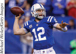
It may help to think of it this way: Andrew Luck is a superb quarterback for the Indianapolis Colts. Let $B$ = the event the Colts win, and let $A$ be the event that Andrew Luck gets injured. The Colts are certainly better with their great quarter-back than without him. So $P (B)$ is greater than $P (B | A)$ , because their chances of winning decrease if Luck gets injured. Because $P (B) \neq P (B given A)$ , the two events $A$ and $B$ are dependent. This makes sense, because the probability of the Colts winning is dependent on whether Andrew Luck gets injured. Now, do the same calculations—this time letting event $C$ be the event that the water boy for the Colts gets injured. It is not likely that the water boy getting injured will affect the Colts’ chances of winning, so that $P (B) = P (B given C)$ . Thus, the events $B$ = Colts win-ning and $C$ = water boy gets injured are independent.

Alternatively, in Step 1 you can find $P$ ( $A$ ) and in Step 2 you can find $P (A given B)$ . Then compare these two quantities for Step 3.

Strategy for Determining Whether Two Events Are Independent

Find $P (B)$ .
Find $P (B given A)$ .
Compare the two probabilities. If they are equal, then $A$ and $B$ are independent events. Otherwise, $A$ and $B$ are dependent events.

Page 275

EXAMPLE 20 Determining whether two events are independent

Table 22 contains a contingency table summarizing the gender and survival status of the passengers and crew of RMS Titanic.

Table 5.55: Table 22 Contingency table of gender and survival status of passengers and crew of RMS Titanic. Notice that when we are given that the person is a female, we may restrict our attention to the females in the table.

	Female	Male	Total
Did not survive	126	1364	1490
Survived	344	367	711
Total	470	1731	2201

Table 5.55: Source: Report on the Loss of the “Titanic” (S.S.). British Board of Trade Inquiry Report (reprint), Allan Sutton Publishing, Gloucester, United Kingdom, 1990.

Suppose our experiment is to select one person at random from the passengers and crew. Define the following events:

$F : Person is a female$
$S : Person survived$

Determine whether events $F$ and $S$ are independent.

Solution

We use the strategy for determining whether two events are independent.

Step 1 Find $P (F) = P (Person is a female)$ . There are 470 females out of a total of 2201 passengers and crew. Thus, $P (F) = 470 / 2201 \approx 0.21$ .
Step 2 We need to find $P (F given S)$ , which is the probability that the person survived, given the person was female. We are told that the person was female, so we may restrict our attention to the females in the table. In other words, our sample space is reduced when we know that the person was a female. Of the 470 females, 344 survived, so that $P (F given S) = 344 / 470 \approx 0.73$ .
Step 3 Because, $P (F) \neq P (F given S)$ , we conclude that $F$ and $S$ are dependent events.

NOW YOU CAN DO

Exercise 33–52.

YOUR TURN#13

In Example 20, determine whether being a male and not surviving are independent.

(The solution is shown in Appendix A.)

Developing Your Statistical Sense

Don’t Confuse Independent Events and Mutually Exclusive Events

It is important to stress the difference between independent events and mutually exclusive events. Mutually exclusive events have no outcomes in common. For two events to be independent means that the occurrence of one does not affect the probability of the other. The concepts are different.

EXAMPLE 21 Gambler's Fallacy

Suppose we have tossed a fair coin 10 times and have observed heads come up every time. Find the probability of tails on the next toss.

Solution

We have observed an unusual number of heads, so we might think that the probability of tails on the next toss is increased. However, the short answer is “Not so.” Successive tosses of a fair coin are independent because the coin has no memory of its previous tosses. Thus, what happened on the first 10 tosses has no effect on the next toss. Probability theory tells us that, in the long run, the proportion of heads and tails will eventually even out if the coin is fair. Therefore, the probability of tails on the next toss is 0.5. This is an example of the Gambler’s Fallacy.

Page 276

3 Multiplication rule

Just as the Addition Rule is used to find probabilities of unions of events, the Multiplication rule is used to find probabilities of intersections of events. Recall the formula for the conditional probability of event $B$ given event $A$ :

$P (B given A) = \frac{P (A and B)}{P (A)} where P (A) \neq 0$

We solve for $P$ ( $A$ and $B$ ) by multiplying each side by $P (A)$ :

$P (A and B) = P (A) \cdot P (B given A)$

Similarly, consider the conditional probability of event $A$ given event $B$ :

$P (A given B) = \frac{P (A and B)}{P (B)} where P (B) \neq 0$

Solving for $P (A and B)$ gives us a second equation for $P (A and B)$ :

$P (A and B) = P (B) \cdot P (A given B)$

The two equations for $P (A and B)$ lead directly to the Multiplication Rule.

Multiplication Rule

$P (A and B) = P (A) \cdot P (B given A) or equivalently P (A and B) = P (B) \cdot P (A given B)$

EXAMPLE 22 Multiplication Rule

According to the Pew Internet and American Life Project,¹¹ 35% of American adults have cell phones with apps, but only 68% of those who have apps on their cell phones actually use the apps. Define the following events:

$A : American adult has a cell phone with apps.$
$U : American adult uses the apps on his or her cell phone.$

Find $P (A)$ .
Find $P$ ( $U$ given $A$ ), the probability that an American adult uses the apps, given that he or she has a cell phone with apps.
Use the multiplication rule to calculate $P (A and U)$ , the probability that an American adult has a cell phone with apps and uses the apps on his or her cell phone.

Solution

According to the study, 35% of American adults have a cell phone with apps. So $P (A)$ = 0.35.
The research says that 68% of those who have apps actually use them, so $P (U given A) = 0.68$ .
Using the Multiplication Rule, we have
$P (A and U) = P (A) \cdot P (U given A) = 0.35 (0.68) = 0.238$

The probability that an American adult has a cell phone with apps and uses them is 0.238.

NOW YOU CAN DO

Exercises 53–58.

Page 277

YOUR TURN#14

Suppose our experiment is to toss a fair die twice. Find the probability of rolling two sixes in a row.

(The solution is shown in Appendix A.)

By the definition of independent events (page 274), when events $A$ and $B$ are independent, $P (A given B) = P (A) or P (B given A) = P (B)$ . Using these identities, we can formulate a special case of the Multiplication Rule. Using $P (A given B) = P (A)$ , we can write the Multiplication Rule as

$P (A and B) = P (B) \cdot P (A | B) = P (B) P (A) = P (A) P (B)$

Equivalently, the Multiplication Rule also states that $P (A and B) = P (A) \cdot P (B given A)$ , but if $A$ and $B$ are independent, $P (B and A) = P (B)$ , so, again, $P (A and B) = P (A) P (B)$ .

Multiplication Rule for Two Independent Events

If $A$ and $B$ are any two independent events, $P (A and B) = P (A) P (B)$ .

EXAMPLE 23 Multiplication Rule for two independent events

Successive spins of the roulette wheel are independent because the wheel does not remember its result from the previous spin. Suppose the experiment is to spin the roulette wheel two times and to bet on red each time. There are 18 red numbers out of a total of 38 num-bers on the wheel. What is the probability that red will occur twice in succession?

Solution

Define the following events:

$A : Roulette wheel comes up red on the first spin.$
$B : Roulette wheel comes up red on the second spin.$

We have the probability of each event given as:

$P (A) = P (B) = \frac{18}{38}$

Then, because the successive spins are independent, the Multiplication Rule for Two Independent Events tells us:

$P (Winning) = P (A and B) = P (A) \cdot P (B) = (\frac{18}{38}) (\frac{18}{38}) \approx 0.2244$

NOW YOU CAN DO

Exercises 59–66.

YOUR TURN#15

For the roulette experiment in Example 23, what is the probability of not getting red on the first spin and not getting red on the second spin?

(The solution is shown in Appendix A.)

Sampling With and Without Replacement

The relationship between two events can be determined by the way the samples are chosen. Two methods of choosing samples are sampling with replacement and sam-pling without replacement.

In sampling with replacement, the randomly selected unit is returned to the population after being selected. When sampling with replacement, it is possible for the same unit to be sampled more than once.

In sampling without replacement, the randomly selected unit is not returned to the population after being selected. When sampling without replacement, it is not possible for the same unit to be sampled more than once.

Page 278

EXAMPLE 24 Sampling with replacement

We draw a card at random from a shuffled deck, observe the card, and return it to the deck. The deck is then reshuffled, and we draw another card at random. What is the probability that both cards we select will be aces?

Solution

Define the following events:

$A : Observe an ace on the first draw.$
$B : Observe an ace on the second draw.$

We want to find $P$ ( $A$ and $B$ ), the probability of observing an ace on the first draw and an ace on the second draw. From the Multiplication Rule, $P (A and B) = P (A) \cdot P (B | A)$ . To find $P (A)$ , recall that there are 4 aces in the deck of 52 cards. It is reasonable to assume that all cards are equally likely to be selected, so using the classical method, $P (B given A) = 4 / 52$ . Similarly, $P (B) = 4 / 52$ .

Next, we need to find $P (B given A)$ , the probability of observing an ace on the second draw, given that we observe an ace on the first draw. Because the deck of 52 cards has not changed (except for shuffling), there are still 52 cards—4 of which are aces. Therefore, $P (B given A) = 4 / 52$ . Thus, the probability that both cards we select will be aces is $P (A and B) = P (A) \cdot P (B given A) = (4 / 52) (4 / 52) \approx 0.0059$ .

Note that $P (B given A) = P (B) = 4 / 52$ . Thus, by the alternative method for deter-mining independence, $A$ and $B$ are independent events when sampling with replacement.

NOW YOU CAN DO

Exercises 67–70.

YOUR TURN#16

For the experiment in Example 24, what is the probability of observing hearts on the first draw and observing hearts on the second draw, if we sample with replacement?

(The solution is shown in Appendix A.)

We can generalize this result as follows.

When sampling with replacement, successive draws can be considered independent.

EXAMPLE 25 Sampling without replacement

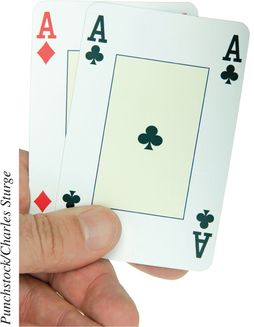
Suppose we alter the experiment in Example 24 as follows: We draw a card at random from a shuffled deck, hold onto the card (do not replace it) while the deck is reshuffled, and then select another card at random. What is the probability that both cards we select will be aces?

Solution

Define events $A$ and $B$ as in Example 24. Again we use the Multiplication Rule to find $P (A and B)$ . The difference in this experiment comes when finding $P (B | A)$ , the probability of observing an ace on the second draw given an ace on the first draw. Once we select the first ace, we do not replace it in the deck. Therefore, when the deck is reshuffled, it has only 51 cards left, only 3 of which are aces. The classical method then gives the probability of observing an ace on the second draw:

$P (B given A) = \frac{number of aces in the deck}{number of cards in the deck} = \frac{3}{51}$

Thus, the probability that both cards we select will be aces is

$P (A and B) = P (A) \cdot P (B given A) = \frac{4}{52} \cdot \frac{3}{51} = \frac{12}{2652} \approx 0.0045$

Page 279

This probability is somewhat less than the probability that both cards will be aces when sampling with replacement. Note that here we found that $P (B given A)$ was not equal to $P (B)$ . Thus, by the alternative method for determining independence, $A$ and $B$ are not independent events; they are dependent events.

NOW YOU CAN DO

Exercises 71–74.

YOUR TURN#17

For the experiment in Example 25, what is the probability of observing hearts on the first draw and observing hearts on the second draw, if we sample without replacement?

(The solution is shown in Appendix A.)

We can generalize this result as follows.

When sampling without replacement, successive draws should be considered dependent.

Note that the Multiplication Rule for Independent Events provides us with an alternative method for determining whether two events are indeed independent.

Alternative Method for Determining Independence

If $P (A) \cdot P (B) = P (A and B)$ , then events $A$ and $B$ are independent.

If $P (A) \cdot P (B) \neq P (A and B)$ , then events $A$ and $B$ are dependent.

EXAMPLE 26 Determining independence using the alternative method

We return to the direct mail marketing data from Example 19, reproduced here in Table 23. Use the alternative method for determining independence to determine whether the following two events are independent:

$R : Responded to direct mail marketing campaign.$
$C : Has a credit card on file.$

Table 5.56: Table 23 Credit card status and marketing response

Response	Credit card on file?
Response	No	Yes	Total
Did not respond	161	79	240
Did respond	17	31	48
Total	178	110	288

Table 5.56: Source: Daniel Larose and Chantal Larose, Data Mining and Predictive Analytics (Wiley Interscience, 2015).

Solution

Using Table 23, we may find the following probabilities:

$\begin{matrix} P (R) = \frac{48}{288} P (C) = \frac{110}{288} P (R a n d C) = \frac{31}{288} \approx 0.1076 \\ P (R) \cdot P (C) = \frac{48}{288} \cdot \frac{110}{288} \approx 0.0637 \end{matrix}$

Because $0.0637 \neq 0.1076$ , we have $P (R) \cdot P (C) \neq P (R and C)$ ; therefore, $R$ and $C$ are dependent.

NOW YOU CAN DO

Exercises 79–84.

Page 280

The next example illustrates the relationship between mutually exclusive events and independence.

EXAMPLE 27 Conditional probability for mutually exclusive events

Suppose two events $A$ and $B$ are mutually exclusive, with $P (A) > 0 and P (B) > 0$ .

Find $P (B given A)$ .
Are events $A$ and $B$ independent or dependent?

Solution

Because $A$ and $B$ are mutually exclusive, $P (B and A) = 0$ . Then

$P (B given A) = \frac{P (A and B)}{P (A)} = 0$

That is, if event A has occurred, then event B cannot occur. This is a natural consequence of events $A$ and $B$ being mutually exclusive.

What Results Might We Expect?

Two events are independent if the occurrence of one does not affect the probability that the other will occur. However, as we saw in (a), if event $A$ occurs, then the probability that event $B$ will occur is 0. Thus, we would expect events $A$ and $B$ to be dependent.
We are given that $P (A) > 0 and P (B) > 0$ . Thus, the product $P (A) \cdot P (B)$ is also greater than 0. However, from (a), $P (A and B) = 0$ . Thus, $P (A) \cdot P (B) \neq P (A and B)$ , and from the alternative method for determining independence, we conclude that events $A$ and $B$ are dependent.

In other words, if two events are mutually exclusive, then they are dependent.

NOW YOU CAN DO

Exercises 85–92.

We can extend the Multiplication Rule to cover $n$ independent events.

Multiplication Rule for n Independent Events

If $A$ , $B$ , $C$ , … are independent events, then $P (A and B and C and \dots) = P (A) \cdot P (B) \cdot P (C) \dots$

EXAMPLE 28 Multiplication rule for $n$ independent events

According to the National Health Interview Survey, 24% of Americans ages 18–44 smoke tobacco. In a random sample of $n = 3$ Americans ages 18–44, find the probability that all three smoke.

Solution

The U.S. Census Bureau estimates that over 100 million Americans are ages 18–44. We will shortly see that, because the sample of 3 is so small compared to the population of over 100 million, it is reasonable to assume that the successive draws are independent. Let $S_{i}$ denote the event that the $i$ th American in the 18–44 age group smokes.

$P (S_{1}) = P (S_{2}) = P (S_{3}) = 0.24$

Page 281

Then, using the Multiplication Rule for $n$ Independent Events,

$P (S_{1} and S_{2} and S_{3}) = P (S_{1}) \cdot P (S_{2}) \cdot P (S_{3}) = (0.24) (0.24) (0.24) = {(0.24)}^{3} = 0.013824$

NOW YOU CAN DO

Exercises 93–100.

YOUR TURN#18

Refer to Example 28. In a random sample of $n = 10$ Americans ages 18–44, find the probability that all 10 smoke.

(The solution is shown in Appendix A.)

Next, we turn to solving an “at least” problem. This involves a technique that uses complements in order to give us a nice shortcut for calculating a probability.

EXAMPLE 29 Solving an “at least” problem

Using information in Example 28, find the probability that, in a random sample of 5 Americans ages 18–44, at least 1 of them smokes.

Solution

The phrase “at least” means that one or more of the five Americans smoke, so the probability we are looking for is:

$P (1 or 2 or 3 or 4 or 5 Americans smoke)$

Now, each of these events is mutually exclusive, meaning that our sample can’t yield exactly 1 American who smokes and exactly 2 Americans who smoke. Thus, by the Addition Rule for Mutually Exclusive Events, the above probability equals:

$P (1 American smokes) + P (2 Americans smoke) + \dots + P (5 Americans smoke)$

Calculating all these probabilities would take a while. So, we can use the probability of the complement we learned earlier to get us a shortcut. Note that “at least 1 American smokes” is the complement of “no Americans smoke.” Then, because the complement rule for probability is: $P (A^{C}) = 1 - P (A)$ , we get:

$\begin{matrix} P (At least 1 of the 5 Americans smokes) \\ = 1 - P (None of the 5 Americans smokes because the events are independent) \\ = 1 - P (1 st doesn' t smoke and 2 nd doesn' t smoke and \dots and 5 th doesn' t smoke) \\ = 1 - P (1 st doesn' t smoke) \cdot P (2 nd doesn' t smoke) \cdot \dots \cdot P (5 th doesn' t smoke) \\ = 1 - {(0.76)}^{5} because P (not smoking) = 0.76 \\ = 0.7464 \end{matrix}$

NOW YOU CAN DO

Exercises 101–104.

YOUR TURN#19

For the experiment in Example 29, find the probability that, in a random sample of four Americans ages 18–44, at least one of them smokes.

(The solution is shown in Appendix A.)

Page 282

4 Approximating Probabilities for Dependent Events

When the sample size is small compared to the population size, we can estimate the probability of a dependent event as if it were independent. The question is: How small is a small sample? We will use the following 1% Guideline.

The 1% Guideline

Suppose successive draws, such as those for a random sample, are being made from a population. If the sample size is no larger than 1% of the size of the population, then the probability of dependent successive draws from the population may be approximated using the assumption that the draws are independent.

EXAMPLE 30 Applying the 1% Guideline

The Gardasil vaccine

In the Section 5.2 exercises, we found the probability that a randomly chosen patient completed the treatment to be $(469 / 1413) \approx 0.3319$ . Suppose we take a random sample of size $n = 2$ patients.

Calculate the probability that both patients complete the treatment, using sampling without replacement.
Confirm that the 1% Guideline applies.
Approximate the probability that both patients complete the treatment using the 1% Guideline.
Find the approximation error by comparing your answers from (a) and (c).

Solution

Define the following events:

$A : First patient completes the treatment$
$B : Second patient completes the treatment$

We have $P (A) = (469 / 1413)$ . Then, given that the first patient completed the treatment, we have, by sampling without replacement, $P (B | A) = (468 / 1412)$ . Then the Multiplication Rule gives us $P (A and B) = P (A) \cdot P (B given A) = (469 / 1413) \cdot (468 / 1412) \approx 0.110012$ .
The sample of size 2 represents $\frac{2}{1413} = 0.0014 = 0.14 %$ of the population. Thus, the 1% Guideline applies, and we may treat the successive draws as independent.
Thus, we can use the Multiplication Rule for Independent Events to solve this problem.
$P (A and B) = P (A) \cdot P (B) = (469 / 1413) (469 / 1413) = 0.110169$
The approximation error, the difference between (a) and (c), is $0.110169 - 0.110012 = 0.000157$ . For most applications, this small approximation error is acceptable.

The 1% Guideline is also helpful when we do not know the size of the population, but may presume that the population is very large compared to the sample size.

NOW YOU CAN DO

Exercises 75–78

5 Bayes’ Rule

When new information becomes available, our estimates of probability need to be revised to reflect the presence of the new information. An English Presbyterian Minister, Thomas Bayes (1702–1761) developed a rule, called Bayes’ rule, for updating previous probabilities using new information to arrive at revised probabilities.

Page 283

Bayes' Rule

For any two events $A$ and $B$ ,

$P (A given B) = \frac{P (A) \cdot P (B given A)}{P (A) \cdot P (B given A) + P (A^{C}) \cdot P (B given A^{C})}$

We apply Bayes’ Rule in the following example.

EXAMPLE 31 Bayes' Rule

The Gardasil vaccine

Table 24 contains a contingency table (crosstabulation) of the variables com-pleted and insurance type for the data set Gardasil.¹²

Table 5.57: Table 24 Contingency table of the variables completed and insurance type

			Insurance type
		Hospital- based	Medical assistance	Military	Private payer	Total
Completed	No	45	220	209	470	944
	Yes	39	55	122	253	469
	Total	84	275	331	723	1413

Define the following events:

$M : Insurance type = Military$
$C : Completed the vaccination treatment$

Use Bayes’ Rule to find the probability that a randomly selected patient used military insurance, given that he or she completed the treatment.

Solution

We are interested in the probability $P (M given C)$ . Substituting $M$ for $A$ and $C$ for $B$ in the formula for Bayes’ Rule, we obtain:

$P (M given C) = \frac{P (M) \cdot P (C given M)}{P (M) \cdot P (C given M) + P (M^{C}) \cdot P (C given M^{C})}$

From Table 24, we have $P (M) = \frac{331}{1413} and P (C given M) = \frac{122}{331}$ . The event $M^{C}$ consists of all other insurance types besides military. So we have $P (M^{C}) = \frac{1082}{1413}$ , and $P (C given M^{C}) = \frac{347}{1082}$ . Thus,

$P (M given C) = \frac{331}{1413} \cdot \frac{122}{331} \frac{331}{1413} \cdot \frac{122}{331} + \frac{1082}{1413} \cdot \frac{347}{1082} = \frac{122}{1413} \frac{122}{1413} + \frac{347}{1413} = \frac{122}{469} \approx 0.26$

Note that this result is confirmed by the direct calculation of $P (M / C)$ using Table 24, which is the single cell of 122 military completers divided by the total number of completers.

NOW YOU CAN DO

Exercises 105–108.

YOUR TURN#20

Using Table 24 and Bayes’ Rule, find the probability that a randomly selected patient used hospital-based insurance, given that he or she completed the treatment.

(The solution is shown in Appendix A.)

Page 284

EXAMPLE 32 The ELISA test for the presence of HIV

The ELISA test is used to screen blood for the presence of HIV. Like most diagnostic procedures, the test is not foolproof.

When a blood sample contains HIV, the ELISA test will give a positive result 99.6% of the time. That is, the false-negative rate, the percentage of tests returning a negative result when the HIV virus is actually present, is $1 - 0.996 = 0.004$ .
When the blood does not contain HIV, the ELISA test will give a negative result 98% of the time. That is, the false-positive rate, the percentage of tests returning a positive result when the HIV virus is not actually present, is $1 - 0.98 = 0.02$ .

A positive result means that the test says that the person has the HIV infection. A negative result means that the test says that the person does not have the virus. The prevalence rate for HIV in the general population is 0.5%. That is, 5 of 1000 persons in the general population have HIV.

Suppose we have samples of blood from 100,000 randomly chosen people.

Problem 1. How many people in the sample of 100,000 have HIV? How many do not?

Solution

The prevalence rate of 0.5% means that $0.005 (100, 000) = 500$ people in the sample have HIV. The remainder—99,500—do not.

Problem 2. A positive result is given 99.6% of the time for blood containing HIV. For the 500 people with HIV, how many positive results will the ELISA test return? How many of the 500 people with HIV will receive a negative result?

Solution

The ELISA test will return a positive result for $0.996 (500) = 498$ of the 500 people. Thus, two people who actually have HIV will receive a test result indicating that they do not have the virus.

Problem 3. A negative result is given 98% of the time for blood without HIV. For the 99,500 people without HIV, how many negative results will the ELISA test return? Positive results?

Solution

The ELISA test will return a negative result for $0.98 (99, 500) = 97, 510$ of the 99,500 people without HIV. The remaining 2%, or 1990 people, will receive positive ELISA test results, even though they do not have the virus.

We can use the counts we found to fill in Table 25.

Table 5.58: Table 25 ELISA test contingency table

	In reality
ELISA test results	Person has HIV	Person does not have HIV	Total
Positive	498	1,990	2,488
Negative	2	97,510	97,512
Total	500	99,500	100,000

Page 285

We will use the information in the ELISA test contingency table to solve Problems 4 and 5. If a person is chosen at random from the sample of 100,000, define the following events:

$A$ : Person has HIV.
$A^{C}$ : Person does not have HIV.
Pos: ELISA test returned positive results.
Neg: ELISA test returned negative results.

Problem 4. What is the probability that a randomly chosen person actually does have HIV, given that the ELISA results are negative? In other words, find $P (A | Neg)$ .

Solution

$P (A given Neg) = \frac{N (A and Neg)}{N (Neg)} = \frac{2}{97, 512} \approx 0.0000205$

Problem 5. What is the probability that a randomly chosen person actually does not have HIV, given that the ELISA test results are positive? In other words, find $P (A^{C} given Pos)$ .

Solution

$P (A^{C} given Pos) = \frac{N (A^{C} given Pos)}{N (Pos)} = \frac{1990}{2488} \approx 0.7998 \approx 0.80$

Developing Your Statistical Sense

Which Error Is More Dangerous?

In Problems 4 and 5, we examined the probabilities of the two ways that the ELISA test can be wrong. Which error do you think is more dangerous? $P (A given Neg)$ represents the probability that HIV is present, even though the ELISA test says otherwise. $P (A^{C} given Pos)$ represents the probability that HIV is not present, even though the ELISA test says it is present. The designers of the ELISA test worked hard to reduce the false-negative rate $P (A given Neg)$ to as low a level as possible. They rightly considered that it is the more dangerous type of error because of the epidemic nature of the illness. A person who receives a false-negative ELISA result could spread the infection further. Therefore, the designers tried to keep this probability as low as they could.

There is a price to be paid, however, which is the high false-positive rate, $P (A^{C} given Pos)$ , a very high 80%. Thus, if a random person receives a positive ELISA test result, the probability that the person does not have HIV is 80%. When the ELISA test comes back positive, a second batch of tests that have a more reasonable false-positive rate is usually administered.