Inferential Statistics
Let’s say that the mean number of physical symptoms (like pain) experienced by the participants in each of the three groups was about the same at the beginning of the health-
Depending on the data, different inferential statistics can be used to answer questions such as the ones raised in the preceding paragraph. For example, t tests are used to compare the means of two groups. Researchers could use a t test, for instance, to compare average energy level at the end of the study in the traditional and alternative groups. Another t test could compare the average energy level at the beginning and end of the study within the alternative group. If we wanted to compare the means of more than two groups, another technique, analysis of variance (often abbreviated as ANOVA), could be used. Each inferential statistic helps us determine how likely a particular finding is to have occurred as a matter of nothing more than chance or random variation. If the inferential statistic indicates that the odds of a particular finding occurring are considerably greater than mere chance, we can conclude that our results are statistically significant. In other words, we can conclude with a high degree of confidence that the manipulation of the independent variable, rather than simply chance, is the reason for the results.
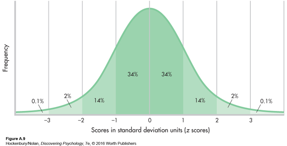
To see how this works, let’s go back to the normal curve for a moment. Remember that we know exactly what percentage of a normal curve falls between any two z scores. If we choose one person at random out of a normal distribution, what is the chance that this person’s z score is above +2? If you look at Figure A.9 (it’s the same as Figure A.5), you will see that about 2.1 percent of the curve lies above a z score (or standard deviation unit) of +2. Therefore, the chance, or probability, that the person we choose will have a z score above + 2 is .021 (or 2.1 chances out of 100). That’s a pretty small chance. If you study the normal curve, you will see that the majority of cases (about 96 percent) fall between –2 and +2 SDs, so in choosing a person at random, that person is not likely to fall above a z score of +2.
When researchers test for statistical significance, they usually employ statistics other than z scores, and they may use distributions that differ in shape from the normal curve. The logic, however, is the same. They compute some kind of inferential statistic that they compare to the appropriate distribution. This comparison tells them the likelihood of obtaining their results if chance alone is operating.
The problem is that no test exists that will tell us for sure whether our intervention or manipulation “worked”; we always have to deal with probabilities, not certainties. Researchers have developed some conventions to guide them in their decisions about whether or not their study results are statistically significant. Generally, when the probability of obtaining a particular result if random factors alone are operating is less than .05 (5 chances out of 100), the results are considered statistically significant. Researchers who want to be even more sure set their probability value at .01 (1 chance out of 100).
Because researchers deal with probabilities, there is a small but real possibility of erroneously concluding that study results are significant; this is called a Type I error. The results of one study, therefore, should never be completely trusted. For researchers to have greater confidence in a particular effect or result, the study should be repeated, or replicated. If the same results are obtained in different studies, then we can be more certain that our conclusions about a particular intervention or effect are correct.
There is a second decision error that can be made—
One final point about inferential statistics. Are the researchers interested only in the changes that might have occurred in the small groups of people participating in the health-
So what did the health-