In this tutorial, we are going to examine one aspect of climate change, carbon dioxide levels. We will look at levels of CO2 in countries and various world regions for the past 50 years.
Part B: Examine the Data Set
Let’s look at some of the climate data from The World Bank at http://data.worldbank.org/indicator/EN.ATM.CO2E.PC . The data given here represent per capita CO2 emissions (in metric tons) in various countries around the world. Create a graph that appropriately represents these data. The following sample table represents just a few countries for which data is available.
Per Capita CO2 Emissions (metric tons)
Year
2005
2006
2007
2008
2009
United States
19.7
19.2
18.3
18.6
17.3
China
4.4
4.9
5.2
5.3
5.8
India
1.3
1.3
1.4
1.5
1.7
Japan
9.7
9.6
9.8
9.5
8.6
Table : Source: The World Bank, http://data.worldbank.org/indicator/EN.ATM.CO2E.PC
1.
Which of these most accurately describes what we need to do with the data?
A.
B.
C.
D.
E.
Correct.
Incorrect.
2.
Based on what you know about graphing, what type of graph is most appropriate for these data?
A.
B.
C.
D.
E.
3.
Which is the dependent variable in this data set, and which axis would it be graphed on?
A.
B.
C.
D.
E.
Correct.
Incorrect.
Part C: Build the Graph
Instructions: Create a graph below. Begin by giving it a relevant title, such as "CO2 Emissions compared". Label the X axis as “Year”, and the the Y axis as "Per Capital CO2 Emissions (metric tons)". Label the Y axis as "Country."
Next, input the actual data into the graph. Each group of data (U.S, China, India, Japan) will be graphed as a line. Students must graph the line with the lowest overall numbers first, followed by the next lowest and so on. The area between each line will then be filled in to create the area graph.
Per Capita CO2 Emissions (metric tons)
Year
2005
2006
2007
2008
2009
United States
19.7
19.2
18.3
18.6
17.3
China
4.4
4.9
5.2
5.3
5.8
India
1.3
1.3
1.4
1.5
1.7
Japan
9.7
9.6
9.8
9.5
8.6
Table : Source: The World Bank, http://data.worldbank.org/indicator/EN.ATM.CO2E.PC
4.
Which country shown on your graph has the greatest increase in per capita CO2 emissions?
A.
B.
C.
D.
Correct.
Incorrect.
Part D: Apply Skills
5.
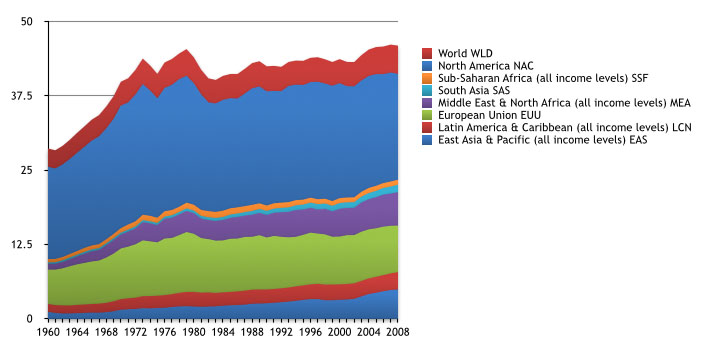
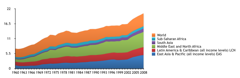
Look at the graph above. What has happened to CO2 levels in each region of the world since 1960?
A.
B.
C.
Correct. CO2 has increased in each world region since 1960.
Incorrect.
6.
According to the graph, which area of the world has contributed least to overall world levels of CO2?
A.
B.
C.
D.
Part D: Apply Skills
Next we add the data for the European Union and North America to the graph.
7.
Based on these data, which region has contributed the most to worldwide increases in CO2 on a per person basis?