EXAMPLE 14![]() The Logistic Population Model
The Logistic Population Model
What behaviors can occur in the logistic model?
For different values of the parameter λ and different starting values for the population fraction, each of the behaviors of Figure 23.12 on page 966 can occur:
- λ=2.8 and starting population fraction x = 0.357 produces the values 0. 357, 0.643, 0.643, …, the pattern shown in the lower graph in Figure 23.12a.
- λ=3.1 and starting population fraction x=0.235 produces the values 0.235, 0. 557, 0.765, 0.558, 0.765, 0.558, …, the pattern shown in the lower graph in Figure 23.12b.
- λ=2.5 and starting population fraction x=0.550 produces the values 0.550, 0. 619, 0.590, 0.605, 0.598, 0.601, 0.599, …, the pattern shown in the lower graph in Figure 23.12c.
In other words, for population growth rates (values of λ) that are fairly close together (2.5, 2.8, 3.1), the population evolves very differently. This is a surprising and nonintuitive conclusion.
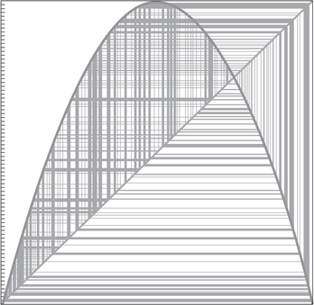
But there is more. For λ=4 and any starting population fraction, the population does not settle down into any of the patterns of Figure 23.12; year after year, it wanders “unpredictably” all over the place (Figure 23.17). This is chaotic behavior: It is deterministic, complex, but—in the long run—unpredictable. In the short run, the behavior is completely predictable. For example, from this year’s population fraction, the equation tells us exactly what next year’s will be. Repeating the use of the equation, we can determine what it will be the following year. But as the years pass, any sense of pattern gets lost in the complexity.