14.5 14.4 Which Divisor Method Is Best?
Why was the supplemental apportionment bill of 1872 enacted? (See Spotlight 14.2 on the preceding page.) Perhaps the goal was to get what was perceived to be a fairer apportionment. Let’s focus on the district populations of the states in the original apportionment bill, which agreed with the Webster and Hamilton methods. Ohio had a population of 2,665,260 and was apportioned 20 seats, so its district population was 133,263. Vermont’s population was 330,551, with 2 seats, for a district population of 165,275.5. This apportionment was advantageous to Ohio, since its district population was 32,012.5 less. Suppose a seat were transferred from Ohio to Vermont. Ohio’s district population would then be
2,665,260÷(20−1)=140,276.8
and Vermont’s would be
330,551÷(2+1)=110,183.7
Now the advantage is to Vermont, by 30,093.1. Since the difference in district populations was reduced by the transfer, it would be fairer to transfer a seat from Ohio to Vermont, if one believes that the fairest apportionment is one that cannot be improved by such a transfer of seats.
Of course, it would not do to reduce Ohio’s apportionment, but if one just gave an extra seat to Vermont, other inequities emerge. The solution is to give additional seats to other states. While it was not necessary to add nine seats (providing one additional seat each to Florida and Vermont would have been sufficient), the supplemented apportionment is optimal in the sense that it is impossible to reduce the difference in district populations between any two states by transferring a seat from one of the states to the other.
The Dean method is a divisor method that minimizes differences in district populations; thus, a Dean apportionment leads to an equitable apportionment in terms of district population. The method was proposed by James Dean (1776–1849) in 1832, in a letter to Senator Daniel Webster. Dean was a mathematics professor who knew Webster when he was an undergraduate at Dartmouth College. The Dean method has never been officially used to apportion seats in the House, but it may have been the source of the supplemental apportionment in 1872. To explore this interesting apportionment method, see Writing Project 2 on page 619.
Self Check 17
According to the 2010 census, the apportionment population of California was 37,341,989 and the state was apportioned 53 seats in the House of Representatives. Montana, with apportionment population 994,416, was apportioned just one seat. The district population of California was 704,565. Determine the district populations that would result if a seat were transferred from California to Montana. Would the difference be less if this transfer took place?
- With the current apportionment, the difference in district populations is in California’s favor by 289,851. If a seat had been transferred from California to Montana, California’s district population would increase to 37,341,989÷52=718,115. Montana’s district population would be 994,416÷2=497,208. The difference, 220,907, is less than the difference before the transfer. Therefore, this apportionment is not equitable by absolute difference in district population. (However, the percentage difference after the transfer, 220,907497,208=44%, is greater than the percentage difference before the transfer, 289,851718,815=40.3%. This was to be expected, because the Hill-Huntington method minimizes percentage differences.)
One way to compare apportionment methods is to investigate bias based on population. The Dean method is known to be biased in favor of states with small populations—but it does provide a way to minimize inequities in district population. There are other ways to measure apportionment inequities between states. For an account of two recent disputes that focused on such inequities, see Spotlight 14.3.
Legal Challenges to Apportionment 14.3
14.3
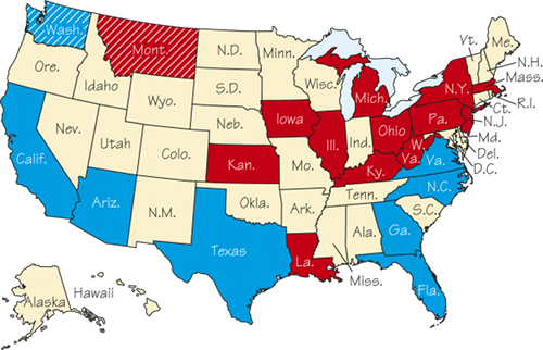
In 1991, the Census Bureau reported the apportionment of congressional seats resulting from the 1990 census. The states colored red on the above map lost representatives, and those in blue gained representatives. New York lost three representatives, and Ohio and Pennsylvania lost two apiece. Montana, whose apportionment decreased from 2 to 1, sustained the greatest percentage loss, and Montana sued to restore the lost seat. As precedents, Montana referred to the two famous cases, Baker v. Carr and Wesberry v. Sanders, in which the U.S. Supreme Court required state legislative and congressional district boundaries to be drawn so as to make district populations equal. Montana argued that the correct apportionment would be the one that met the Baker and Wesberry criterion of having district populations as nearly equal as possible, and asked the court to require the Census Bureau to recompute the apportionments using the Dean method. This would have resulted in the transfer of a congressional seat from Washington to Montana.
The Montana case proceeded concurrently with another federal lawsuit, Massachusetts v. Mosbacher, which asked the Federal District Court to order the apportionment to be calculated by the Webster method. if Massachusetts had won this suit, a seat would have been transferred to it from Oklahoma (see Exercise 42 on page 617). The apportionments of Montana and Washington would not have changed.
In U.S. Department of Commerce v. Montana, the Supreme Court unanimously rejected Montana’s claim. The opinion of the court, written by Justice John Paul Stevens, pointed out that intrastate districts, which were the subject of the Baker and Wesberry cases, could be equalized in population by drawing district boundaries correctly. Because congressional districts can’t cross state lines, some inequity is inevitable in congressional apportionment. The opinion conceded that there were alternative apportionment methods but concluded that the choice of apportionment method must be left to Congress.
Representative Share DEFINITION
Let a be the apportionment given to a state whose population is p. The quotient a÷p is called the representative share for that state. It represents the share of a congressional seat given to each citizen of the state.
Ideally, every state would have the same representative share. This is impossible, just as we cannot expect each state to have the same district population. We can measure how close a given apportionment is to being ideal by using district population as the standard of comparison, or we can compare representative shares. If state X had a greater representative share than state Y, we would see if the difference between their representative shares would be reduced if we transferred a seat from the more advantaged state, X, to the state Y. If it is impossible to reduce the difference in representative shares between any pair of states, then the apportionment is equitable by representative share.
One might ask if the Dean method, which minimizes differences in district populations, minimizes differences in representative share too. The answer provided by the following theorem is no; it is the Webster method that minimizes differences in representative share.
Webster Method and Representative Share THEOREM
If a seat is transferred from one state to another in an apportionment that was calculated by the Webster method, the absolute difference between their representative shares will not decrease.
Here’s the reasoning behind this theorem. Suppose that the divisor used in a Webster apportionment is d. The apportionment, a, given to a state with population p is the whole number nearest to pd. The representative share is ap, which is the closest multiple of 1p to 1d. Hence, with the Webster apportionment, all states have representative shares as close as possible to 1d. A transfer of a seat from one state to another cannot move either states’ representative shares closer to 1d, and thus not closer to each other.
For example, if seats in a parliament are apportioned by using a Sainte-Laguë table, then the apportionment is equitable from the point of view of representative share. This means that among all apportionments of parliament, this particular apportionment gives all voters—as nearly as possible—equal shares of a seat in the parliament.
EXAMPLE 17![]() Inequity in the 113th Congress?
Inequity in the 113th Congress?
The 2010 census reported the following apportionment populations: North Carolina, 9,565,781, and Rhode Island, 1,055,247. The states were apportioned 13 seats and 2 seats in Congress, respectively. Would it have been fairer to give North Carolina 14 of the 15 seats between them? We will calculate the district populations and representative shares for both apportionments and make a comparison.
With 13 seats to North Carolina, the district populations are 9,565,781÷13=735,829 for North Carolina and 1,055,247÷2=527,634 for Rhode Island. The representative share for the states are 13÷9.565781 million=1.359 seats per million for North Carolina and 2÷1.055247 million=1.895 seats per million for Rhode Island. With a smaller district population and a larger representative share, Rhode Island has the advantage with this apportionment. The bottom line: Rhode Island’s district populations are 208,195 smaller than North Carolina’s, and Rhode Island’s representative share is 0. 536 seats per million larger than North Carolina’s.
Table 14.17 summarizes what we have calculated so far and compares the results with those that would be obtained if North Carolina had been apportioned 14 seats to Rhode Island’s 1. With the 14-1 apportionment, North Carolina would have the advantage. Its district size would have been 371,977 less than Rhode Island’s. This would be a greater discrepancy than exists with the 13-2 apportionment. On the other hand, North Carolina’s representative share would have been 0.516 seats per million greater than Rhode Island’s—a smaller discrepancy than exists with the 13-2 apportionment!
| Dist Pop | Rep Share | |||
|---|---|---|---|---|
| State | 13-2 | 14-1 | 13-2 | 14-1 |
| NC | 735,829 | 683,270 | 1.35901 | 1.46355 |
| Rl | 527,634 | 1,055,247 | 1.89529 | 0.94765 |
| Difference | 208,195 | 371,977 | 0.53628 | 0.51590 |
Edward V. Huntington, a mathematics professor at Harvard University, pointed out that if percentage differences are compared instead of absolute differences, then district population and representative share would give identical comparisons of apportionments4—and he suggested a compromise.
Absolute and Percentage Difference DEFINITION
Given two positive numbers A and B, with A>B, the absolute difference is equal to A−B and the percentage difference is equal to the quotient A−BB×100%. In computing the percentage difference between two numbers, the lesser of the two numbers goes in the denominator.
Self Check 18
The world record for the men’s 100-meter race, 9.6 seconds, was set in 2009 by Usain Bolt. A century earlier, the record was 10.6 seconds, held by Knut Lindberg.
- Find the percentage difference between these records.
- The percentage difference in the records is 10.6−9.69.6=10.42%.
- Find the average speed, in meters per second, for both runners.
- Bolt’s average speed was 100 meters9.6 seconds=10.417 meters per second. Lindberg’s average speed was 100 meters10.6 seconds=9.434 meters per second.
- Find the percentage difference in the speeds of the runners.
- The percentage difference in speeds is 10.417−9.4349,434=10.42%.
EXAMPLE 18![]() Percentage Inequity in the 113th Congress
Percentage Inequity in the 113th Congress
Let’s refer to Table 14.17 again and recalculate the “bottom line” as percentage differences. For example, for the percentage difference in district population with the “13-2” apportionment, we would divide the absolute difference, 208,195, by the lesser district population, which is Rhode Island’s, 527,634. The result is 39.46%. You can calculate the remaining entries and obtain the following.
| Dist Pop | Rep Share | |||
|---|---|---|---|---|
| 13-2 | 14-1 | 13-2 | 14-1 | |
| Percentage difference | 39.46% | 54.44% | 39.46% | 54.44% |
You can see that the percentage differences in district population and representative share are the same, as Professor Huntington said that they would be, and that in terms of these, the “13-2” apportionment, where North Carolina gets 13 seats and Rhode Island gets 2, is preferred.
To optimize apportionment by the percentage difference criterion for equity, Professor Huntington and Joseph Hill, a statistician from the Census Bureau, designed a new divisor method. It has been used to apportion seats in the U.S. House of Representatives after each decennial census since 1940.
The Hill-Huntington Method
Like the Jefferson, Webster, and Dean methods, the Hill-Huntington method calculates the apportionment by rounding apportionment quotients. The only difference between the four divisor methods is in the rounding procedure.
The Hill-Huntington rounding procedure is related to the geometric mean.
Geometric Mean DEFINITION
The geometric mean of two positive numbers A and B is equal to the square root of their product, √A×B.
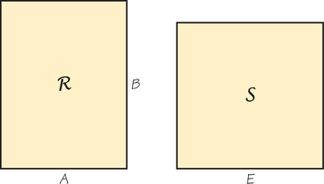
Consider the rectangle ℛ, displayed in Figure 14.1. The area of ℛ is the product of the lengths A and B, or A×B. The geometric mean of A and B is equal to the length E of the edge of a square S with the same area as ℛ. For example, suppose A=4 and B=9. The area of ℛ equals 4×9=36. The square with the same area as ℛ would have edge E=6, since 62=36. In general, E=√A×B.
Self Check 19
Find the geometric mean of 5 and 20.
- √5×20=10
Hill-Huntington Rounding DEFINITION
Given a number q that is not negative, let q* be the geometric mean of ⌊q⌋ and ⌈q⌉; that is,
q*=√⌊q⌋×⌈q⌉
This q* is called the Hill-Huntington rounding point for q. The Hill-Huntington rounding of a number q is equal to ⌊q⌋ if q<q* but is equal to ⌈q⌉ if q≥q*.
EXAMPLE 19![]() Hill-Huntington Rounding
Hill-Huntington Rounding
Suppose that q=7.485. Jefferson and Webster would round 7.485 down to 7. Because ⌊q⌋=7 and ⌈q⌉=7, the rounding point is q*=√56=7.483, approximately. Since q>q*, Hill-Huntington rounds q up to get 8.
The procedure for calculating the Hill-Huntington apportionment is similar to the Webster procedure.
Hill-Huntington Apportionment PROCEDURE
- Make a table showing the quota for each state and the Hill-Huntington rounding point for each quota.
- Calculate the Hill-Huntington rounding of each quota.
- Add the rounded quotas from Step 2. If their sum is equal to the house size, they are the apportionment.
- If the sum of the rounded quotas is not equal to the house size, then compute apportionment quotients, using trial divisors that are greater than the standard divisor if the sum of the Hill-Huntington rounded quotas is greater than the house size, and smaller than the standard divisor if the sum is smaller than the house size.
- Round the apportionment quotients from Step 4 and calculate the sum. If the sum is equal to the house size, the job is finished; otherwise, repeat Step 4.
If a state’s (possibly adjusted) quota q is less than 1, then ⌊q⌋=0. Hence q*=√0×1=0. It follows that the Hill-Huntington rounding of any quota less than 1 is equal to 1. This proves the following theorem, which distinguishes the Hill-Huntington method from the Hamilton, Jefferson, and Webster methods. (Each of these can be modified to guarantee that each state receives at least one seat.)
No Zero Apportionments THEOREM
The Hill-Huntington method is incapable of apportioning zero seats to any state.
EXAMPLE 20![]() Rounding Summands
Rounding Summands
Let’s use the Hill-Huntington method to round each summand in
0.10 +1.43+2.47=4.00
Each summand is the quota, for the standard divisor is 1. The rounding points are as follows:
For numbers between0 and 11 and 22 and 3Approximate Hill-Huntington rounding point0√2=1.41√6=2.45
Each summand is greater than its corresponding rounding point, so all are rounded up, resulting in a too large sum: 1+2+3 = 6. We’ll need to choose a divisor larger than 1; let’s try 2. The apportionment quotients are
0.10÷2=0.05, 1.43÷2=0.715, 2.47÷2=1.235
The first two apportionment quotients are between 0 and 1, and so they are rounded to 1; the third is below the rounding point between 1 and 2, so it too rounds to 1. The sum, 3, is too small.
Let’s try again with a smaller divisor, d=1.5. The new apportionment quotients are
0.10÷1.5=0.067, 1.43÷1.5=0.953, 2.47÷1.5=1.647
The first two apportionment quotients are still between 0 and 1, so they round to 1. The third is greater than the rounding point between 1 and 2, so it rounds to 2. Therefore the Hill-Huntington rounding of this sum is
1+1+2=4
Self Check 20
Use the Hill-Huntington method to round the percentages:
98.1%+1.8%+0.1%=100.0%
(You may use 1.007 as the divisor.) Does the apportionment satisfy the quota condition?
By Hill-Huntington, all numbers between 0 and 1 are rounded to 1, all numbers between 1.414 and 2 are rounded to 2, and 98.1 would be rounded to 98. Thus, the rounded percentages are 98%+2%+1%=101%. We have to use a divisor greater than the standard divisor (which is 1) to reduce the sum. As suggested, we’ll take 1.7 as the divisor. The apportionment quotients are 98.1%÷1.007=97.42%, 1.8%÷1.007=1.79%, and 0.1%÷1.007=0.099%. The rounding point for numbers between 97 and 98 is
√97×98=97.4987
Thus, 97.42% is rounded down to 97%, and the other two percentages are rounded up. The Hill-Huntington rounding,
97%+2%+1%=100%
violates the quota condition because the first percentage is apportioned less than its lower quota.
An apportionment is equitable by percentage differences (in either representative share or district population) if it is impossible to reduce the percentage difference in representative share (or district population) between any pair of states by taking a seat from one and giving it to the other. The advantage of the Hill-Huntington method is that it provides a way to determine the apportionment that is equitable by percentage differences.
Equity and the Hill-Huntington Method THEOREM
An apportionment is equitable by percentage differences if and only if it is the same as the apportionment that is produced by the Hill-Huntington method.
EXAMPLE 21![]() Percent Effort
Percent Effort
Faculty members at a certain university must state the percentage of their time spent in several activities. Professor Worktorule has requisitioned five stopwatches to keep track of her activities. Table 14.18 shows, in its left columns, what she recorded over the course of one week.
| Effort Category |
Effort (in minutes) |
Quota | Rounding Point |
Tentative Apportionment |
|---|---|---|---|---|
| Instruction | 300 | 8.33% | 8.485 | 8% |
| Lecture prep | 705 | 19.58% | 19.494 | 20% |
| Indep. Study | 31 | 0.86% | 0.000 | 1% |
| Research | 2475 | 68.75% | 68.498 | 69% |
| Committees | 89 | 2.47% | 2.449 | 3% |
| Totals | 3600 | 100% | — | 101% |
The professor is too busy to convert the data into percentages—which the university requires in whole numbers with sum 100%—so we’ll do it, using the Hill–Huntington method. (She requested this method because she wanted the result to display a nonzero percentage for each of her activities.) As with any percentage apportionment problem, the house size is 100, so the standard divisor—one percentage unit—is the population, 3600, divided by 100, or 36 minutes. Table 14.18 shows in its right columns, the quotas, the rounding points, and the tentative apportionment, obtained by rounding the quotas up or down, depending on whether the quota is above the rounding point or not.
Because too many “seats” were awarded, we’ll try divisors larger than the standard divisor, 36. The results are shown in Table 14.19. The first divisor we tried, 36.5, produced 98 “seats” too few. The left column under that divisor shows the corresponding apportionment quotients (AQ), obtained by dividing the minutes devoted to each activity by that divisor. The middle column shows the Hill-Huntington rounding points (RP) for the apportionment quotients, and the right column displays the Hill-Huntington tentative apportionment (TA). To increase the number of “seats” apportioned, the next trial divisor must be closer to 36 (but more than 36). We tried the divisor 36.2 and found that 99 “seats” were apportioned. Our third trial divisor was 36.1 (not shown in the table), which apportioned 101 “seats”—too many. The divisor we needed was therefore between 36.1 and 36.2. We set the divisor equal to 36.15, and the table shows that exactly 100 “seats” were apportioned. The right column of Table 14.19 displays the percentages that Professor Worktorule should put into her effort report.
| Divisors | ||||||||||
|---|---|---|---|---|---|---|---|---|---|---|
| 36.5 | 36.2 | 36.15 | ||||||||
| Cat. | Pop | AQ | RP | TA | AQ | RP | TA | AQ | RP | TA |
| Inst | 300 | 8.219 | 8.485 | 8 | 8.287 | 8.485 | 8 | 8.299 | 8.485 | 8 |
| Prep | 705 | 19.315 | 19.494 | 19 | 19.475 | 19.494 | 19 | 19.502 | 19.494 | 20 |
| Ind St | 31 | 0.849 | 0.000 | 1 | 0.856 | 0.000 | 1 | 0.858 | 0.000 | 1 |
| Research | 2475 | 67.808 | 67.498 | 68 | 68.370 | 68.498 | 68 | 68.465 | 68.498 | 68 |
| Com | 89 | 2.438 | 2.449 | 2 | 2.459 | 2.449 | 3 | 2.462 | 2.449 | 3 |
| Totals | 3600 | 98 | 99 | 100 | ||||||
EXAMPLE 22![]() The 435th Seat
The 435th Seat
The Webster and Hill-Huntington methods give almost the same apportionments, based on the 2010 census. The only difference is that the Webster method apportions the last seat to North Carolina, while the Hill-Huntington method gives it to Rhode Island.
The standard divisor s is the apportionment population of the United States, 309,183,463, divided by the number of seats, 435. Thus, s=710,767. The quotas, obtained by dividing the states’ populations by s, are 9,565,781÷s=13.458 for North Carolina and 1,055,247÷s=1.485 for Rhode Island. With the Webster method, both quotas would be rounded down and only 434 seats would be apportioned. If we reduce the divisor to 708,000, North Carolina’s quotient becomes 13.51, which will be rounded up, and Rhode Island’s quotient is 1.49, which will be rounded down. North Carolina will get 14 seats, and Rhode Island will get 1.
With the Hill-Huntington method, the rounding point for numbers between 13 and 14 is q*=√13×14=13.49, which is greater than North Carolina’s quota. The rounding point for numbers between 1 and 2 is q*=√2=1.41, which is less than Rhode Island’s quota. Therefore, North Carolina’s quota is rounded down to get its apportionment, 13, and Rhode Island’s quota is rounded up to get its apportionment, 2, with the Hill-Huntington method.
The 435th seat was in play between Michigan and Arkansas as a result of the 1940 census, and the resulting dispute led to the permanent adoption of the Hill-Huntington method for the apportionment of seats in the House of Representatives (see Spotlight 14.4).
We have seen that the Jefferson method is biased in favor of populous states and that the Webster method is not biased in regard to state population size. It’s natural to ask if the Hill-Huntington method exhibits any bias with respect to state population.
A divisor method will show bias in favor of large states when the quotas are adjusted by using a divisor that is smaller than the standard divisor. If the quotas must be adjusted downward—that is, a divisor larger than the standard divisor is used—small states are favored. Because the rounding point for the Webster method is halfway between whole numbers, it is just as likely for the divisor to be smaller than the standard divisor as it is for it to be larger.
For any positive number q, the rounding point used by the Hill-Huntington method is closer to ⌊q⌋ than to ⌈q⌉ (see Exercise 40 on page 617). This means that a random number q is more likely to be above the rounding point, and thus rounded up to ⌈q⌉, than it is to be less, and thus rounded down to ⌊q⌋. The difference between the Webster and Hill-Huntington ways of rounding is not significant for relatively large numbers. For example, the Hill-Huntington rounding point between 50 and 51 is 50.498. Therefore, a number q between 50 and 51 will be rounded up to 51 by Hill-Huntington if it is larger than 50.498. The Webster method would round q to 51 if q≥50.500.
Mathematics and Politics: A Strange Mixture 14.4
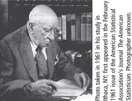
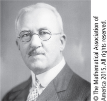
The first American to consider apportionment from a theoretical point of view was Walter Willcox (1861–1964), who strongly advocated the Webster method and had computed the apportionment of the 78th Congress in 1902. His arguments convinced Congress to use the Webster method again in 1912. In 1911, Joseph Hill, a statistician at the Census Bureau, proposed the Hill-Huntington method—with the endorsement of Edward V. Huntington, a mathematics professor at Harvard.
In 1920, the two methods were in competition. There were significant differences in the apportionments determined by the two methods, and the result was Washington gridlock: No apportionment bill passed during the decade, and the 1912 apportionment was retained throughout the 1920s. In preparation for the 1930 census results, the National Academy of Sciences formed a committee of distinguished mathematicians to study apportionment. In 1929, the committee endorsed the Hill-Huntington method.
The 1930 census was remarkable in that the apportionments calculated by the Webster method were the same as the Hill-Huntington apportionments. Therefore, the House of Representatives was reapportioned, but the method used could be claimed to be either one of the competing methods. The coincidence was almost repeated in the 1940 census, but there was one difference: The Hill-Huntington method gave the last seat to Arkansas, while Webster’s method gave it to Michigan. At the time, Michigan was a predominantly Republican state and Arkansas was in the Democratic column. The vote on the apportionment bill split strictly along party lines, with Democrats supporting the Hill-Huntington method and Republicans voting for the Webster method. Because the Democrats had the majority, the Hill-Huntington method became law.
The differences are more significant when rounding smaller numbers. Hill-Huntington rounds all numbers between 0 and 1 up to 1; Webster rounds only the numbers between 0.500 and 1 up to 1. When the Hill-Huntington method is used for apportionment, the sum of the tentative apportionments is more likely to exceed the house size than it is to be less, especially if there are many states with small populations. Therefore, the Hill-Huntington method is likely to use a divisor larger than the standard divisor. This favors the less populous states.
In conclusion, the Webster method is the only divisor method that is unbiased regarding population size, and it minimizes differences between representative shares. Although the Webster method is capable of violating the quota condition, it is the divisor method least likely to do so.
For apportionment of seats in the U.S. House of Representatives by the Webster method, a slight modification is needed, because no state can receive a zero apportionment. The rounding point for quotas less than 1 is set to 0, rather than 0.5.
There are situations where other apportionment methods could be considered. See Exercise 46 (page 617) to explore ways to make teaching assignments.