23.2 23.1 Growth Models for Biological Populations
We encountered geometric growth models for savings accounts in Chapter 21. Growth is proportional to the amount present, and such growth is expressed in terms of compound interest and its formula.
We now use a geometric growth model to estimate the sizes of human populations. In addition to the rate of natural increase—the annual birth rate minus the annual death rate—we must take into account net immigration. The sum of the natural rate of increase and net immigration, in the terminology of financial models, is the effective rate of growth.
Birth, death, and migration rates rarely remain constant for long, so projections must be made with care. In the short run, however, predictions based on the model may be useful. Let’s apply this model to two questions about the population of the United States.
EXAMPLE 1![]() Predicting the U.S. Population
Predicting the U.S. Population
The U.S. population increased at an average effective growth rate of 0.77% per year (including immigration) to 321 million at mid-2015. What would be the anticipated population at mid-2020? What would it be if the effective rate of growth changes to 1% per year, or to 0.5% per year?
We apply the compound interest formula with initial population size (“principal”) 321 million. Using one year as the compounding period and the compound interest formula A=P(1+r)n, where n=5, the projected population size in mid-2020 for a rate r=0.0077 is
population in 2020=(population in 2015)×(1+growth rate)5=321,000,000(1+0.0077)5=321,000,000(1.03909)≈334,000,000
Because of the limited accuracy of the estimates of population and growth rate, we round off the final answer. The result of a calculation can’t be more precise than the ingredients; we round back to millions because that was the precision of our original data.
Using the same formula, a growth rate of 1% per year leads to a population of 337 million, while a growth rate of 0.5% per year yields 329 million.
Self Check 1
Why is a formula from banking relevant here?
- The compound interest formula is not just for banking but for any "population" that increases geometrically (exponentially).
So an uncertainty of about one-fourth of one percentage point (0.23–0.27%) in the growth rate has major implications, even over fairly short time horizons. The presence or absence of 3 to 5 million people would have a significant impact on our social and economic systems, in terms of need (or lack thereof) of daycare centers, schools, and products for babies and children. (About one- third of population growth in the United States is projected to come from net immigration.)
At the other end of the age distribution, much of the concern over long-range funding of the Social Security and Medicare programs results from uncertainties over birth and immigration rates. Figure 23.1a gives a graph of the U.S. population in 2015, structured by age and sex, and Figure 23.1b does the same for Nigeria.
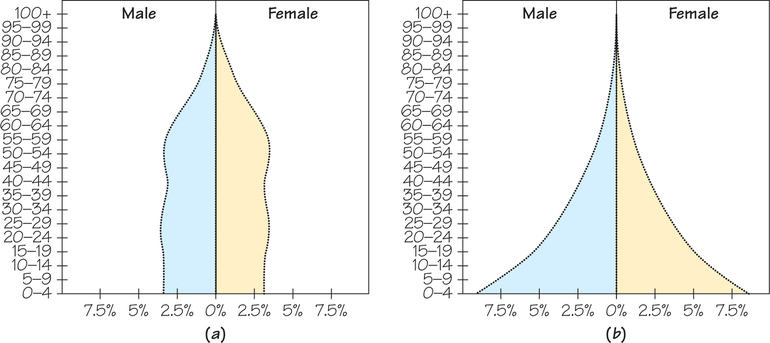
Rates of increase in most developing nations are much higher than in industrialized nations. At a rate of 2.8%, the population of Nigeria, Africa’s most populous country, will grow from 184 million in mid-2015 to 240 million in mid-2025, a shocking increase of one-third—and 60 million people!—in only 10 years. Such projections raise concern over providing sufficient food and resources for all people.
It is not just the number of people that is crucial, but also the population structure. In poorer countries, the proportion of the population over 60 years of age will be 20% by 2050, compared with 8% now; in Japan, where the overall population is expected to decline by one-sixth by then, it will be more than 40%.
Limitations on Growth
A population that keeps adding a fixed percentage each year, like a bank account accumulating compound interest, would eventually grow to astronomical numbers. But no biological population can continue to increase without limit (see Spotlight 23.2). Its growth is eventually constrained by the availability of resources such as food, shelter, and psychological and social “space.” There may be a maximum population size that can be supported by the available resources, the carrying capacity of the environment.
Carrying Capacity DEFINITION
The carrying capacity of an environment is the maximum population size that it can support indefinitely with the available stream of resources.
As the population increases toward the carrying capacity—which we will denote by K—the growth rate decreases.
12 Billion by 2050—or Only 9 Billion? 23.2
23.2
How many people can the world hold? Are developing countries heading for a population disaster? Will falling fertility play havoc with Social Security in the United States? Will aging result in 50% of Japanese being over 60 in 2100?
Potential answers come from mathematical modeling of the future, using predictions of trends. The best analyses suggest a probability distribution over a range of estimates. They project separately by age, gender, education, and other characteristics. They try to factor in improvements in agriculture, spread of diseases (e.g., HIV), changes in urbanization, increases in economic aspirations, and the potential for climate change (e.g., from global warming).
A basic concept is total fertility rate (TFR), the average number of births per woman. Absent catastrophes (such as war or epidemic), a rate of 2.1 continues a population at the same size. A model that assumes a value above 2.1 will predict an increasing population; one that assumes a value below 2.1 will predict a dwindling one. Most of the world’s population growth will occur in the lesser-developed countries, whose TFR values are well above 2.1 (e.g., it is 4.8 for Africa as a whole). However, all countries in Europe have TFR values below 2.1; without immigration, they will lose population and struggle with fewer workers to provide social benefits to the elderly. The value for the United States is 1.86, but the population is increasing nevertheless because of immigration.
China’s situation illustrates demographic momentum. Its fertility rate has been below the replacement level for 20 years and is now about 1.5. To some extent, this reduction may be due to the government’s policy of one child per family, though economic gains and widespread education of women may be more responsible. However, the number of women in the childbearing years was (and still is) so large that China’s population will continue to grow until 2020. If present trends continue, it will then decline by 100 million by 2040 and by 250 million more by 2060. Such a swift and large decline would have disastrous economic and social consequences.
Sophisticated models try to assess how the TFR will vary with changing social circumstances. The most important single factor impacting fertility is education of women. There is a strong negative association between level of education and TFR, and the effect can be very large: In India and China, women with some college education have, on average, only half as many children as women with no education. Hence, a country’s policies about education, and their success, may directly impact future population levels.
As we have revised this book for successive editions, we have seen population projections change. The estimates have decreased, because fertility rates have declined. The key questions are how to model such declines, whether they will continue, and how they will adapt to other world changes. In Spotlight 21.1 (page 878), we saw Malthus’s oversimplified prediction that arithmetic growth in food supplies would limit the geometric increase of human populations. Some demographers now think that population growth will remain a serious problem in some parts of the world but that global population may stabilize or even decline after 2050.
How many people the world will have depends on how well we as a world conserve the environment, distribute food, provide jobs, produce and consume energy, and make other critical decisions about our money and resources. The key concern is the quality of life of all people. Political and economic events in far corners of the world, and even natural disasters—such as the tsunami in the Indian ocean at the end of 2004 and the earthquakes in Haiti in 2010 and Fukushima, Japan, in 2011—impact us all. Neglecting problems faced by increasing numbers of poor people provides no security, peace, or moral refuge for anyone.
The carrying capacity is the long-range capacity to support the population, so the population could exceed it for short periods of time. This could happen either because the population grows very rapidly and surges above the carrying capacity or because the food supply suddenly decreases, thus temporarily lowering the carrying capacity, as happens to deer and other animals in winter. The discrete logistic model is a simple model that provides excellent predictions for some populations.
Logistic Model DEFINITION
The discrete logistic model for population growth takes carrying capacity into account by reducing the population by a term that measures how close the population size P is to the carrying capacity K. The population grows from a population of Pn in year n to Pn+1 in year (n+1) according to
Pn+1=Pn+rPn(1−PnK)=(1+r)Pn−rPnPnK=(1+r)Pn−rKP2n
where r is the natural rate of increase when the population is small.
When the population Pn is close to 0, then Pn/K is also close to 0, the factor (1−pnK) is close to 1, and we have Pn+1≈(1+r)Pn, which is exponential growth. However, when the population Pn is close to K, then Pn/K is close to 1 and provides a “brake” on further population growth.
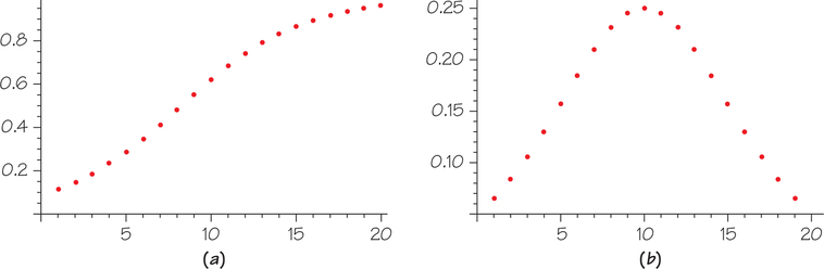
Starting from small numbers, a population following the logistic model will at first grow exponentially. Then its rate of increase will slow to a linear pace before tapering off as the population approaches the carrying capacity. Figure 23.2 shows such growth, with the population measured in terms of a fraction of its carrying capacity.
In fact, the fastest growth of the population—corresponding to the steepest slope of the population curve—occurs when the population is at the halfway point K/2 toward the carrying capacity K.
EXAMPLE 2![]() Logistic Model for the U.S. Population
Logistic Model for the U.S. Population
How well does the historical U.S. population fit a logistic model?
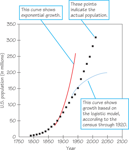
The U.S. population from 1790 to 1950 closely followed a logistic model with r=0.031=3.1%, P=population in 1790=3,900,000, and K=201 million. In the first decades after 1790, the population was a small fraction of this carrying capacity, and it grew at close to the rate r=3.1% per year (a rate higher than in many developing nations today). By 1920, the U.S. population had reached 106 million, and the growth rate had slowed by about one-half, to 1.5% per year (see Figure 23.3).
The 2015 U.S. population of 321 million far exceeds the carrying capacity of 201 million that the model suggested. Why? What was wrong with the model? The structure of the U.S. population changed, from a large proportion of people making their living on family farms to a highly urbanized society. The average number of children per family shrank. As the structure changed, the model based on assumptions of the prior structure gradually became invalid. A logistic model to the data through 2010 suggests a carrying capacity in excess of 400 million, which leaves room for growth toward the 420 million projected by the Census Bureau in 2050.
Self Check 2
One data point in Figure 23.3 is noticeably lower than you might otherwise expect from the indicated trend. Why do you think that is so?
- The data point for 1940 reflects a low birthrate during the Great Depression in the 1930s.
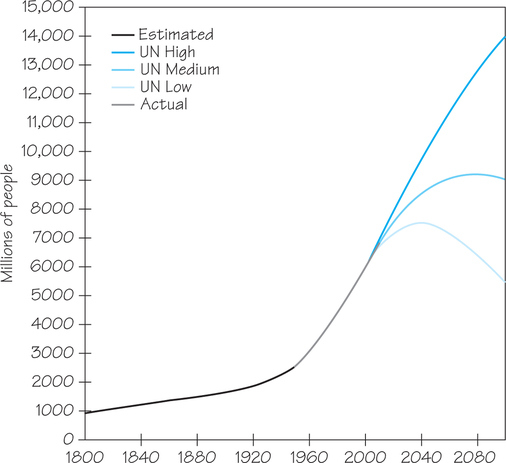
What about the world population? Figure 23.4 shows the historical trend—which does not show any sign of tapering off yet toward a carrying capacity—and three projections for the future. By the time you may retire, say, in the 2050s, you will know which came true.
The logistic model applies not only to population growth limited by carrying capacity but also to modeling the spread of a technology or product, such as smartphones or flat-screen plasma TVs. Consider again Figure 23.2 (page 948) and think of the population as a population of smartphone sales. Initially, sales are slow. Then they begin to climb rapidly. Finally, as the market gets saturated, sales slow. We will see in the next section that the logistic model can apply also to exhaustion of nonrenewable resources.