2 Business Efficiency

2.2 2.1 Hamiltonian Circuits

The concept is named for the Irish mathematician William Rowan Hamilton (1805–1865), who was one of the first to study it. We now know that the concept was discovered somewhat earlier by Thomas Kirkman (1806–1895), a British minister with a penchant for mathematics.

The concepts of Euler and Hamiltonian circuits are similar in that both forbid reuse. An Euler circuit forbids the reuse of edges, while a Hamiltonian circuit forbids the reuse of vertices. However, it is far more difficult to determine which connected graphs possess Hamiltonian circuits than to determine which connected graphs have Euler circuits. Using the concepts of Euler circuit and Hamiltonian circuit in practical applications in the real world involves actually being able to find such circuits in large graphs. As we saw in Chapter 1, looking at the valences of vertices tells us whether a connected graph has an Euler circuit, but we have no such simple method for telling whether or not a graph has a Hamiltonian circuit.

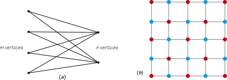
Some special classes of graphs are known to have Hamiltonian circuits, and some special classes of graphs are known to lack them. For example, here is a method for constructing an infinite family of graphs where each graph in the family cannot have a Hamiltonian circuit. Construct a vertical column of m vertices and a parallel column of n vertices, where m is bigger than n, as shown in Figure 2.2a. The figure illustrates a typical case where and . Now join each vertex on the left in the figure to every vertex on the right. As m and n vary, we get a family of different graphs.

No graph obtained in this manner can have a Hamiltonian circuit. If a Hamiltonian circuit existed, it would have to alternately include vertices on the left and right of the figure. This is not possible because the number of vertices on the left and right are not the same. It is unlikely that a method will ever be found to easily determine whether or not a graph has a Hamiltonian circuit based on theoretical results developed in computer science. If Hamiltonian circuits were easy to find in any graph at all, many applied problems could be solved in a less costly way.

In many urban operations research situations, “grid graphs” such as the one in Figure 2.2b are of interest. If we wanted an efficient route (circuit) to inspect traffic surveillance cameras located at urban street intersections, we would need to find a Hamiltonian circuit for the graph in Figure 2.2b. Note that in going from one vertex to another, we move from a vertex of one color to a vertex of the other color. Since colors would alternate in a Hamiltonian circuit, it follows that the number of vertices of each color would have to be the same if there is a Hamiltonian circuit in this graph. Since the number of vertices of the two colors is not the same, there is no Hamiltonian circuit and, hence, no fully efficient route for inspecting the traffic control cameras.

The Hamiltonian circuit problem itself has many applications. This is not unusual in mathematics. Often mathematics used to solve a particular real-world problem leads to new mathematics that suggests applications to other real-world situations. One class of problems to which we can apply Hamiltonian circuits is vacation planning.

It may seem that delivering mail in a cheap and timely manner should not be that hard. However, finding the best way to deliver mail over a variety of environments, rural, suburban, and urban, is very complex. How should a large geographic area be divided into smaller sections? Should each mail carrier use a truck as a “depot” to resupply small amounts of mail for delivery or should there be deposit boxes on street corners? Mathematics can be used to find answers to such questions.

Figure 2.2: Figure 2.2 (a) An example of one graph from a family of graphs that has no Hamiltonian circuit. The number of vertices m on the left is chosen to be greater than the number of vertices n on the right. The case and is shown. (b) A graph used to model a portion of a city. Since the graph reflects the block structure of the city, it is known as a “grid graph.”

Express mail and parcel post delivery companies need to make complicated patterns of deliveries and pick-ups. To do this, they need to know driving distances between the various geographical locations involved. Using this information, together with driving times, they can use mathematics to cut costs and to make the pick-ups and deliveries on time.

EXAMPLE 1 Vacation Planning

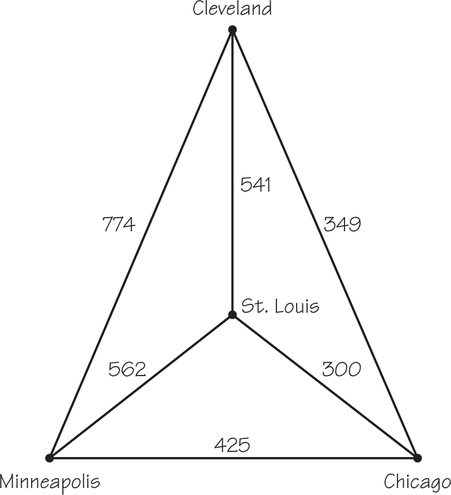
Let’s imagine that you are a college student studying in Chicago. During spring break, you and a group of friends have decided to take a car trip to visit other friends in Minneapolis, Cleveland, and St. Louis. there are many choices as to the order of visiting the cities and returning to Chicago, but you want to design a route that minimizes the distance you have to travel. Presumably, you also want a route that cuts costs, and you know that minimizing distance will minimize the cost of gasoline for the trip. Similar problems with different complications would arise for bus, railroad, or airplane trips.

Imagine now that the internet has provided you with the intercity driving distances between Chicago, Minneapolis, Cleveland, and St. Louis. We can construct a graph model with this information, representing each city by a vertex and the legs of the journey between the cities by edges joining the vertices. TO construct the model, we add a number called a weight to each graph edge, as in Figure 2.3. In this example, the weights represent the distances between the cities, each of which corresponds to one of the endpoints of the edges in the graph. (in other examples the weight might represent a cost, time, satisfaction rating, or profit.) We want to find a minimum-cost tour that starts and ends in Chicago and visits each other city only once. Using our earlier terminology, what we wish to find is a minimum-cost Hamiltonian circuit—a Hamiltonian circuit with the lowest possible sum of the weights of its edges.

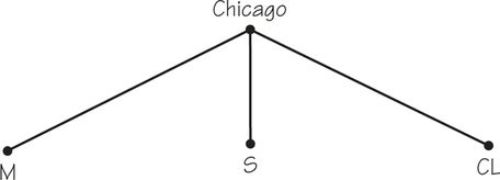
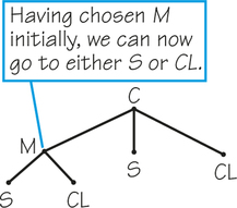
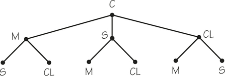
Steps 2 and 3 of the algorithm are straightforward. thus, we need worry only about Step 1, generating all the possible Hamiltonian circuits in a systematic way. TO find the Hamiltonian tours, we use the method of trees, as follows: Starting from Chicago, we can choose any of the three cities to visit after leaving Chicago. The first stage of the enumeration tree is shown in Figure 2.4. if Minneapolis is chosen as the first city to visit, then there are two possible cities to visit next, Cleveland and St. Louis. the possible branchings of the tree at this stage are shown in Figure 2.5. In this second stage, however, for each choice of first city to visit, there are two choices from this city to the second city to visit. This would lead to the diagram in Figure 2.6.

Figure 2.3: Figure 2.3 Road mileages between four cities.

Finding a Minimum-Cost Hamiltonian Circuit PROCEDURE

How can we determine which Hamiltonian circuit has minimum cost? There is a conceptually easy algorithm, or a step-by-step process like a recipe in cooking, for solving this problem:

Generate all possible Hamiltonian tours (starting from Chicago).
Add up the distances on the edges of each tour.
Choose a tour with total distance being a minimum, that is, as small as possible.

Figure 2.4: Figure 2.4 First stage in finding vacation-planning routes.

Figure 2.5: Figure 2.5 Part of the second stage in finding vacation-planning routes.

Figure 2.6: Figure 2.6 Complete second stage in finding vacation- planning routes.

Having chosen the order of the first two cities to visit, and knowing that no revisits (reuses) can occur in a Hamiltonian circuit, we have only one choice left for the next city. From this city, we return to Chicago. The complete tree diagram showing the third and fourth stages for these routes is given in Figure 2.7.

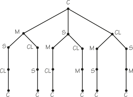
Figure 2.7: Figure 2.7 Completed enumeration of routes using the method of trees for the vacation-planning problem.

Notice, however, that because we can traverse a circular tour in either of two directions, the paths shown in the tree diagram of Figure 2.7 do not correspond to different Hamiltonian circuits. For example, the leftmost path (C–M–S–CL–C) and the rightmost path (C–CL–S–M–C) represent the same Hamiltonian circuit. Thus, among what appear to be six different paths in the tree diagram, only three in fact correspond to different Hamiltonian circuits. These three distinct Hamiltonian circuits are shown in Figure 2.8.

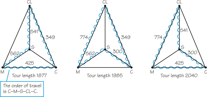
Figure 2.8: Figure 2.8 The three Hamiltonian circuits for the vacation-planning problem of Figure 2.3.

Note that in generating the Hamiltonian circuits, we disregard the distances involved. We are concerned only with the different patterns of carrying out the visits. To find the optimal, or best, route, however, we must add up the distances on the edges to get each tour’s length and select a tour whose total length is smallest. Figure 2.8 shows that the optimal tour is Chicago, Minneapolis, St. Louis, Cleveland, Chicago. The length of this tour is 1877 miles, which saves 163 miles over the longest choice of tour.

The method of trees is not always as easy to use as our example suggests. Instead of doing our analysis for four cities, consider the general case of n cities. The graph model similar to that in Figure 2.3 would consist of a weighted graph with n vertices, with every pair of vertices joined by an edge.

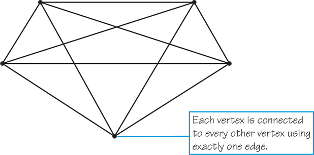
Complete Graph DEFINITION

A graph is called complete if there is exactly one edge between each pair of vertices in the graph.

A complete graph with five vertices is illustrated in Figure 2.9. The graph in Figure 2.3 is a weighted complete graph with four vertices.

Figure 2.9: Figure 2.9 A complete graph with five vertices. Every pair of vertices is joined by an edge.

Fundamental Principle of Counting

How many Hamiltonian circuits are in a complete graph of n vertices? We can solve this problem by using the same type of analysis that we used in the method of trees. The method of trees is a visual application of the fundamental principle of counting, a procedure for counting outcomes in multistage processes. Using this procedure, we can count how many patterns occur in a situation by looking at the number of ways in which the component parts can occur. For example, if Jack has 10 shirts and 4 pairs of trousers, he can wear shirt-pants outfits. Each shirt can be worn with any of the pants. (This can be verified by drawing a tree diagram, but such a diagram is cumbersome for big numbers.)

The Fundamental Principle of Counting DEFINITION

In general, the fundamental principle of counting can be stated this way: If there are a ways of choosing one thing, b ways of choosing a second after the first is chosen,…, and z ways of choosing the last item after the earlier choices, then the total number of choice patterns is .

Note that each choice cannot depend on a prior choice for this count to be valid. When choosing which of the 10 shirts and 4 pants to wear, Jack does not depend on the pants he chooses or the other way around. Therefore, he can make choices.

EXAMPLE 2 Counting

Here are some examples of how to use the fundamental principle of counting:

In a restaurant, there are 4 kinds of soup, 12 entrees, 6 desserts, and 3 drinks. How many different four-course meals can a patron choose? the four choices can be made in 4, 12, 6, and 3 ways, respectively. Hence, applying the fundamental principle of counting, there are possible meals.
In a state lottery, a contestant gets to pick a four-digit number that does not contain a zero followed by an uppercase or lowercase letter. How many such sequences of digits and a letter are there? Each of the four digits can be chosen in 9 ways (i.e., 1, 2,…, 9), and the letter can be chosen in 52 ways (i.e., A, B,…, Z plus a, b,…, z). Hence, there are possible patterns.
A corporation is creating a musical logo consisting of four different ordered notes from the scale C, D, E, F, G, A, and B. How many logos are there to choose from? the first note can be chosen in 7 ways, but because reuse is not allowed, the next note can be chosen in only 6 ways. the remaining two notes can be chosen in 5 and 4 ways, respectively. Using the fundamental principle of counting, musical logos are possible. if reuse of notes is allowed, logos are possible

Let’s now return to the problem of enumerating Hamiltonian circuits for the complete graph with n vertices. The city visited first after the home city can be chosen in ways, the next city in ways, and so on, until only one choice remains. Using the fundamental principle of counting, there are routes. The exclamation mark in is read “factorial” and is shorthand notation for the product . For example, .

As we saw in Figure 2.7, pairs of routes correspond to the same Hamiltonian circuit because one route can be obtained from the other by traversing the cities in reverse order. Thus, although there are possible routes, there are only half as many, or , different Hamiltonian circuits. Now, if we have only a few cities to visit, Hamiltonian circuits can be listed and examined in a reasonable amount of time. Analysis of a six-city problem would require generation of tours. But for, say, 25 cities, is approximately . Even if these tours could be generated at the rate of 1 million per second, it would take almost 10 billion years to generate them all. Because it would take so long to solve large vacation-planning problems using this method, it is sometimes referred to as a brute force method (i.e., trying all the possibilities). Computer scientists and engineers have made it possible to market faster and faster computers. However, governments and businesses need to solve larger-scale problems; say, for example, finding a Hamiltonian circuit in a graph with 10,000 vertices. If the methods one knows for solving such problems are not much better than brute force, then it’s unlikely that even these faster computers can optimally solve large versions of such problems. Mathematicians and computer scientists are actively seeking procedures that will significantly improve our ability to solve large versions of important problems.