2.4 2.3 Helping Traveling Salesmen
Because the traveling salesman problem arises so often in situations where the associated complete graphs would be very large, we must find a faster method than the brute force method we have described. One intuitive idea is to try to visit nearby locations sooner. Recall that our goal is to find the minimum-cost vertex tour that forms a Hamiltonian circuit.
Nearest-Neighbor Algorithm PROCEDURE
Starting from the home city, first visit the nearest city, then visit the nearest city that has not already been visited. We return to the start city when no other choice is available. This approach is called the nearest-neighbor algorithm.
EXAMPLE 3![]() Applying the Nearest-Neighbor Algorithm
Applying the Nearest-Neighbor Algorithm
Applying this algorithm to the TSP in Figure 2.3 quickly leads to the tour of Chicago, St. Louis, Cleveland, Minneapolis, and Chicago, with a length of 2040 miles. Here is how this tour is determined. Because we are starting in Chicago, there is a choice of going to a city that is 425, 300, or 349 miles away. Because the smallest of these numbers is 300, we next visit St. Louis, which is the nearest neighbor of Chicago not already visited. At St. Louis, we have a choice of visiting next cities that are 541 or 562 miles away. Hence, Cleveland, which is nearer (541 miles), is visited. To complete the tour, we visit Minneapolis and return to Chicago, thereby adding 774 and 425 miles to the length of the tour. The total length of the tour is 2040 miles.
The nearest-neighbor algorithm is an example of a greedy algorithm because at each stage a best (greedy) choice, based on an appropriate criterion, is made. Unfortunately, this is not the optimal tour, which we saw was C–M–S–CL–C, for a total length of 1877 miles. Making the best choice at each stage may not yield the best “global” solution. However, even for a large TSP, one can always find a nearest-neighbor route quickly.
EXAMPLE 4![]() Applying the Nearest-Neighbor Algorithm Revisited
Applying the Nearest-Neighbor Algorithm Revisited
Figure 2.10 again illustrates the ease of applying the nearest-neighbor algorithm, this time to a weighted complete graph with five vertices. Starting at vertex A, we get the tour ADECBA (cost 2800) (Figure 2.10a). Note that the nearest-neighbor algorithm starting at vertex B yields the tour BCADEB (cost 3050) (Figure 2.10b).
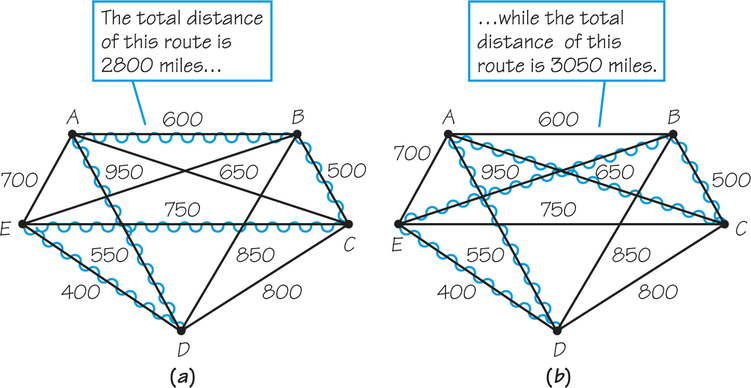
This example illustrates that a nearest-neighbor tour can be computed for each vertex of the complete graph being considered and that different nearest-neighbor tours can be obtained starting at different vertices. Thus, even though we may seek a tour starting at a particular vertex—say, A in Figure 2.10—because a Hamiltonian circuit can be thought of as starting at any of its vertices, we can just as easily apply the nearest-neighbor procedure starting at vertex B (rather than at A). The Hamiltonian circuit we get can still be thought of as beginning at vertex A rather than B. Even for complete graphs with a large number of vertices, it would still be faster to apply the nearest-neighbor algorithm for each vertex and pick the cheapest of the tours generated (though such a tour might not be optimal) than to apply the brute force method.
Self Check 1
Apply the nearest-neighbor algorithm to the graph in Figure 2.10a starting at vertex D. What is the cost of the associated tour?
- DEABCD; cost=3000.
We now consider a different approach to the TSP that might find a good solution quickly.
Sorted-Edges Algorithm PROCEDURE
Start by sorting or arranging the edges of the complete graph in order of increasing cost (or, equivalently, arranging the intercity distances in order of increasing distance). Then at each stage select an edge that has not been previously chosen of least cost that (1) never requires that three used edges meet at a vertex (because a Hamiltonian circuit uses up exactly two edges at each vertex) and (2) never closes up a circular tour that doesn’t include all the vertices. This algorithm is called the sorted-edges algorithm.
EXAMPLE 5![]() Applying the Sorted-Edges Algorithm
Applying the Sorted-Edges Algorithm
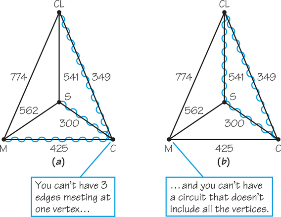
Applying the sorted-edges algorithm to the TSP in Figure 2.3 works as follows: First, the six weights on the edges listed in increasing order would be 300, 349, 425, 541, 562, and 774. Because the cheapest edge in this sorted list is 300, this is the first edge we select for the tour we are building. Next we add the edge with weight 349 to the tour. The next-cheapest edge would be 425, but using this edge together with those already selected would result in having three edges at a vertex (Figure 2.11a), which is not consistent with having a Hamiltonian circuit. Hence, we do not use this edge. The next-cheapest edge, 541, used together with the edges already selected, would create a circuit (see Figure 2.11b) that does not include all the vertices. Thus, this edge, too, would be skipped over. However, we are able to add the edges 562 and 774 without either creating a circuit shorter than one including all the vertices or having three edges at a vertex. Hence, the tour we arrive at is Chicago, St. Louis, Minneapolis, Cleveland, and Chicago. Again, this solution is not optimal because its length is 1985. Note that this algorithm, like the nearest-neighbor, is greedy.
EXAMPLE 6![]() Applying the Sorted-Edges Algorithm Revisited
Applying the Sorted-Edges Algorithm Revisited
Although the edges selected by applying the sorted-edges method to the example in Figure 2.3 are connected to each other at every stage, this does not always happen. For example, if we apply the sorted-edges algorithm to the graph in Figure 2.10a, we build up the tour first with edge ED (400) and then edge BC (500), which do not touch. The edges that are then selected are AD,AB, and EC, giving the circuit EDABCE, which is the same as the nearest-neighbor circuit starting at vertex A. Note we must sort numbers in order to find 5 edges.
Self Check 2
Apply the sorted-edges algorithm to the graph in Figure 2.12 on page 52. What is the cost of the associated tour?
- The edges are added in the order DE, DA, AB, BC, and CE. One way to represent this tour is ABCEDA, and the cost of the tour is 4.8.
NP-Complete Problems 2.1
2.1
Steven Cook, a computer scientist at the University of Toronto, showed in 1971 that certain computational problems are equivalently difficult. this class of problems, now referred to as NP-complete problems, has the following characteristic: if a “fast” algorithm for solving one of these problems could be found, then a fast method would exist for all these problems.
In this context, “fast” means that as the size n of the problem grows (the number of cities gives the problem size in the TSP), the amount of time needed to solve the problem grows no more rapidly than a polynomial function in n. (A polynomial function has the form aknk+ak−1nk−1+⋯a1n+a0.) On the other hand, if it could be shown that any problem in the class of NP-complete problems required an amount of time that grows faster than any polynomial (an exponential function, such as 3n, is an example of a function that grows faster than any polynomial) as the problem size increased, then all problems in the NP-complete class would share this characteristic. The TSP, along with a wide variety of other practical problems, is known to be NP-complete. it is widely believed that large versions of these problems cannot be solved quickly. Furthermore, the security of some recent cryptographical systems relies on the hope that large NP-complete problems are actually as time consuming to solve as they appear to be. The Clay Foundation is offering a $1 million prize for determining whether NP-complete problems are truly computationally hard. The prize is still unclaimed! Researchers are also exploring whether the development of new approaches to computer design, such as quantum computing, will offer faster ways to solve very difficult problems.
Many “quick-and-dirty” methods for solving the TSP have been suggested; while some methods give an optimal solution in some cases, none of these methods guarantees an optimal solution. Surprisingly, most experts believe that no efficient method that guarantees an optimal solution for the TSP will ever be found (see Spotlight 2.1).
Recently, mathematical researchers have adopted a somewhat different strategy for dealing with TSPs. If finding a fast algorithm to generate optimal solutions for large problems is unlikely, perhaps we can show that the quick-and-dirty methods, usually called heuristic algorithms, come close enough to giving optimal solutions to be important for practical use. For example, suppose we could prove that the nearest- neighbor heuristic was never off by more than 25% in the worst case or by more than 15% in the average case. For a medium-sized TSP, we would then have to choose whether to spend a lot of time (or money) to find an optimal solution or instead to use a heuristic algorithm to obtain a fairly good solution. Investigators at AT&T Research have developed many remarkably good heuristic algorithms. The best-known guarantee for a heuristic algorithm for a TSP is that it yields a cost no worse than one and a half times the optimal cost. Interestingly, this heuristic algorithm involves solving a Chinese postman problem (see Chapter 1), for which a “fast” algorithm is known to exist.
Throughout our discussion of the TSP, we have concentrated on the goal of minimizing the cost (or time) of a tour that visited each of a variety of sites once and only once. However, the subtle issues that arise in specific real-world situations (or that provide a contrast between seemingly similar situations) are the things that make mathematical modeling exciting. For example, suppose the TSP situation is to pick up day campers and take them to and from the camp. The camp wants to minimize the total length of time that the bus needs to pick up the campers. The parents of the campers, however, may want to minimize the time their children spend on the bus. For some problems, the tour that minimizes the mean (average) time that a child spends on the bus may not be the same tour that minimizes the total time of the tour. (Specifically, if the bus first picks up the child who lives the farthest from the camp, and then picks up the other children, this may yield a relatively short time on the bus for the kids but a relatively long time for the tour itself.) Mathematicians return to examine these subtleties between problems at a later time, after the basic structure of the main problem itself is well understood. It is in this way that mathematics continues to grow, explore new ideas, and find new applications.