EXAMPLE 7 Cable TV Service

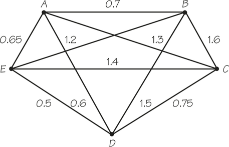
Imagine that cable TV (CT) service will be set up on one large university campus. The graph in Figure 2.12 shows the possible links that might be included in the CT network, with each edge showing the cost in hundreds of thousands of dollars to create that particular link. To send video between two locations, a direct cable link is not necessary because it is possible to send a video indirectly via another site. Thus, in Figure 2.12, sending a video from A to C could be achieved by sending the video from A to B, from B to E, and from E to C, provided the links AB, BE, and EC are part of the network. We assume that the cost of relaying a video, compared with the cost of the direct communication link, is so small that we can neglect this amount. The problem that concerns us, therefore, is to provide service between any pair of locations in a way that minimizes the total cost of the links.

53

Our first guess at a solution is to put in the cheapest possible links between locations first, until all sites could send video to any other site. Such an approach is analogous to the sorted-edges method that was used to study the traveling salesman problem. in our example, if the cheapest links are added until all locations are joined, we obtain the connections shown in Figure 2.13a.

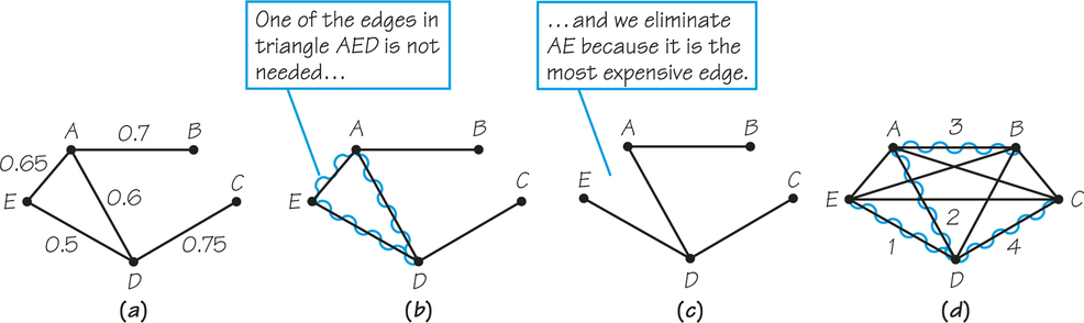
The links were added in the order ED,AD,AE,AB,DC. However, because this graph contains the circuit ADEA (wiggly edges in Figure 2.13b), it has redundant edges: We can still send videos between any pair of sites using relays after omitting the most expensive edge in the circuit—AE. After an edge of a circuit is deleted, a video can still be relayed among the sites of the circuit by sending signals the long way around. After AE is deleted, videos going from A to E can be sent via D (Figure 2.13c). These ideas constitute a procedure developed by Joseph Kruskal (1928-2010) in 1956.

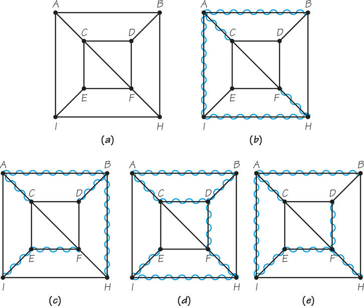
In Kruskal’s procedure, as in the sorted-edges method for the TSP, the edges that are added need not be connected to each other until the end. A subgraph formed in this way is a tree; that is, it consists of one piece and contains no circuits. it also includes all the vertices of the original graph. A subgraph that is a tree and that contains all the vertices of the original graph is called a spanning tree of the original graph.

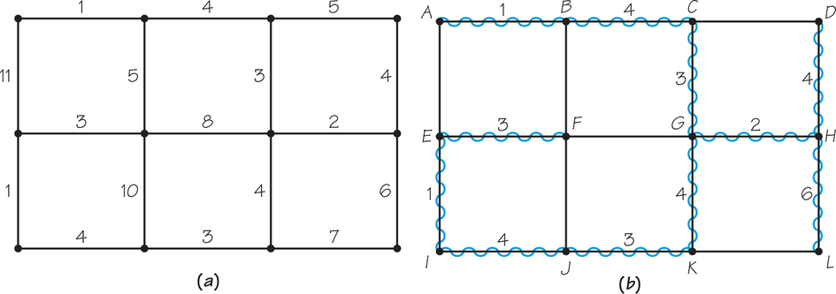
To understand these concepts better, consider the graph G in Figure 2.14a. The wiggly edges in Figure 2.14b constitute a subgraph of G that is a tree (because it is connected and has no circuit), but this tree is not a spanning tree of G because the vertices D and E are not included. On the other hand, the wiggly edges in Figure 2.14c and 2.14d show subgraphs of G that include all the vertices of G but are not trees because the first is not connected and the second contains a circuit. Figure 2.14e shows a spanning tree of G; the wiggly edges are connected and contain no circuit, and every vertex of the original graph is an endpoint of some wiggly edge.

54

Apply Kruskal’s algorithm to find a minimum-cost spanning tree for the graph in Figure 2.3 (page 43). What is the cost associated with the tree you find?

Although long-distance calls are now routine, it takes great expertise and careful planning for a company like AT&T to handle its vast amounts of telephone traffic. Rich Wetmore was district manager of AT&T’s Communications Network Operations Center in Bedminster, New Jersey. Here are his responses to questions about how AT&T handles its huge volumes of long-distance traffic and how it tracks its operations to keep things running smoothly.

How do you make sure that a customer doesn’t run into a delayed signal when attempting a long-distance call?

We monitor the performance of our AT&T network by displaying data collected from all over the country on a special wallboard. The wallboard is configured to tell us if a customer’s call is not going through because the network doesn’t have enough capacity to handle it.

That’s when we step in and take control to correct the problem. The typical control we use is to reroute the call. instead of sending the customer’s call directly to its destination, we’ll route it via a third city—to someplace else in the country that has the capacity to complete the call.

It would seem that routing via another city would take longer. Is the customer aware of this process?

Routing a call via a third city is entirely transparent [imperceptible] to the customer. I’m an expert about the network, and even when i make a phone call, I have no idea how that individual call was routed. it’s transparent both in terms of how far away the other person sounds and in how quickly the telephone call gets set up. With the signaling network we use, it takes milliseconds for switching systems to “talk” to each other to set up a call. So the fact that you are involved in a third switch in some distant city is something you would never know.

You want to be sure to keep costs down while supplying enough service to customers. So how do you balance company benefits with customer benefit?

In terms of making the network efficient, we want to do two things. First, we want our customers to be happy with our service and for all their calls to go through, which means we must build enough capacity in the network to allow that to happen. Second, we want to be efficient for stockholders and not spend more money than we need to for the network to be at the optimum size.

There are basically two costs in terms of building the network. There is the cost of switching systems and the cost of the circuits that connect the switching systems. Basically, you can use operations-research techniques and mathematics to determine cost trade-offs. it may make sense to build direct routing between two switching systems and use a lot of circuits, or maybe to involve three switching systems, with fewer circuits between the main two, and so on.

In the study of ancient manuscripts, different manuscripts of the same book are available, even though the original manuscript upon which they are based has been lost. Examples of this include Euclid’s Elements and Chaucer’s Canterbury Tales. What interests scholars is reconstructing the relationships between the manuscripts and the common ancestors of the manuscripts, even when some of the ancestors are now missing.

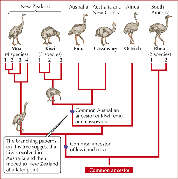
Similarly, perceptual psychologists may be interested in which colors people perceive as being closely related and comparing these perceptions with those of people who are color-blind. Linguists are interested in the connections between languages that seem very different today, but have some words that are similar. Finally, in studying different species, biologists are interested in determining which species are more closely related to each other, including species known only in fossil form, and constructing a “tree” of life that shows which species were ancestors of others.

Reconstructions of this kind are made possible by using graph theory, specifically using the graph theory concept of a tree. The value of the graph theory in these and many other situations lies in using the distance between pairs of vertices in the tree as a way of reflecting the closeness of the relationships that pairs of manuscripts, pairs of colors, or pairs of species have. The distance between two vertices in a tree is the sum of the weights along the one path that joins the two vertices. If there are no weights on the edges, the distance is the number of edges in the path. In some reconstruction problems, a special vertex of the tree called the root is singled out. This root plays the role of the original common ancestors, and distances to the root are of critical interest.

In the case of species, trees of family relatedness were traditionally constructed based on similarities of bones and physical appearance. With the discovery of molecular biology, many new avenues have been opened up. We can now draw trees of relatedness based on an organism’s genetic material, DNA, or the proteins that the DNA codes for. The traditional trees based on physical traits often show different species as being more closely related than trees based on newer molecular biological approaches. These differences cause scholars to focus on how to resolve the discrepancies and thereby reach a deeper understanding of the unity of life.