3.5 3.4 Bin Packing
Suppose you plan to build a wall system for your books, CDs, DVDs, and stereo set. This project requires 24 wooden shelves of various lengths: 6, 6, 5, 5, 5, 4, 4, 4, 4, 2, 2, 2, 2, 3, 3, 7, 7, 5, 5, 8, 8, 4, 4, and 5 feet. The lumberyard, however, sells wood only in boards of length 9 feet. If each board costs $8, what is the minimum cost to buy sufficient wood for this wall system?
Because all shelves required for the wall system are shorter than the boards sold at the lumberyard, the largest number of boards needed is 24, the precise number of shelves needed for the wall system. Buying 24 boards would, of course, be a waste of wood and money because several of the shelves you need could be cut from one board. For example, pieces of length 2, 2, 2, and 3 feet can be cut from one 9-foot board, assuming no loss of wood is created by the cutting process.
To make the ideas we develop more flexible, we think of the boards as bins of capacity W (9 feet in this case) into which we will pack (without overlap) n weights (in this case, lengths) whose values are w1, … , wn, where each wi≤W. We wish to find the minimum number of bins into which the weights can be packed. In this formulation, the problem is known as the bin-packing problem.
Bin-Packing Problem DEFINITION
The bin-packing problem involves finding the minimum number of bins of weight capacity W into which weights w1, w2, … , wn (each less than or equal to W) can be packed without exceeding the capacity of the bins.
At first glance, bin-packing problems may appear unrelated to the machine-scheduling problems we have been studying. However, there is a connection.
Let’s suppose we want to schedule independent tasks so that each machine working on the tasks finishes its work by time W. Instead of fixing the number of machines and trying to find the earliest completion time, we must find the minimum number of machines that will guarantee completion by the fixed completion time (W). Despite this similarity between the machine-scheduling problem and the bin-packing problem, the discussion that follows will use the traditional terminology of bin packing.
By now, it should come as no surprise to learn that no one knows a fast algorithm that always picks the optimal (smallest) number of bins (boards). In fact, the bin-packing problem belongs to the class of NP-complete problems (see Spotlight 2.1 on page 51), which means that most experts think it unlikely that any fast optimal algorithm will ever be found. Relatively good algorithms for problems that come up in actual applications are known.
Bin-Packing Heuristics
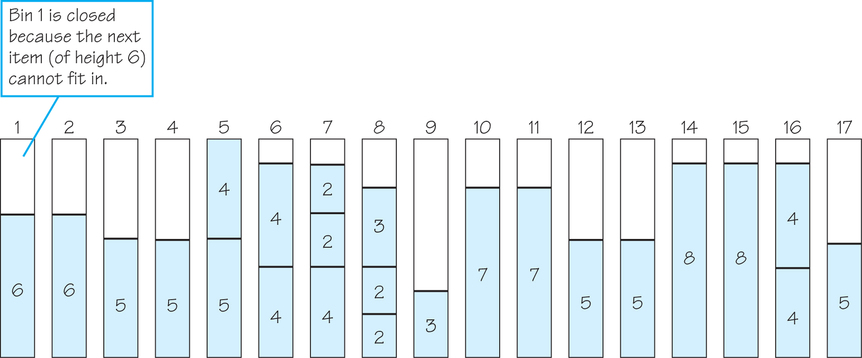
We will think of the items to be packed, in any particular order, as constituting a list. In what follows we will use the list of 24 shelf lengths given for the wall system. We will consider various heuristic algorithms, namely, methods that can be carried out quickly but cannot be guaranteed to produce optimal results. Probably the easiest approach is simply to put the weights into the first bin until the next weight won’t fit, and then start a new bin. (Once you open a new bin, don’t use leftover space in an earlier, partially filled bin.) Continue in the same way until as many bins as necessary are used.
The resulting solution is shown in Figure 3.19. This algorithm, called next fit (NF), has the advantage of not requiring knowledge of all the weights in advance. Only the remaining space in the bin currently being packed must be remembered. The disadvantage of this heuristic is that a bin packed early on may have had room for small items that come later in the list.
Our wish to avoid permanently closing a bin too early suggests a different heuristic—first fit (FF): Put the next weight into the first bin already opened that has room for this weight. If no such bin exists, start a new bin. Note that a computer program to carry out first fit would have to keep track of how much room was left in all the previously opened bins. For the 24 wall-system shelves, the FF algorithm would generate a solution that uses only 14 bins (see Figure 3.20) instead of the 17 bins generated by the NF algorithm.
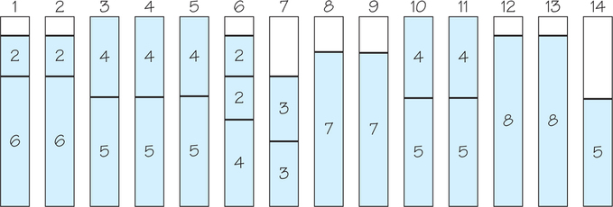
If we are keeping track of how much room remains in each partially filled bin, we can put the next item to be packed into the bin that currently has the most room available. This heuristic will be called worst fit (WF). The name worst fit refers to the fact that an item is packed into a bin with the most room available, that is, into which it fits “worst,” rather than into a bin that will leave little room left over after it is placed in that bin ("best fit"). The solution generated by this approach looks the same as that shown in Figure 3.20. Although this heuristic also leads to 14 bins, the items are packed in a different order. For example, the first item of size 2, the tenth item in the list, is put into bin 6 in worst fit, but into bin 1 in first fit.
Decreasing-Time Heuristics
One difficulty with all three of these heuristics is that large weights that appear late in the list can’t be packed efficiently. Therefore, we should first sort the items to be packed in order of decreasing size, assuming that all items are known in advance. We can then pack large items first and the smaller items into leftover spaces. This approach yields three new heuristics: next-fit decreasing (NFD), first-fit decreasing (FFD), and worst-fit decreasing (WFD). Here is the original list sorted by decreasing size: 8, 8, 7, 7, 6, 6, 5, 5, 5, 5, 5, 5, 4, 4, 4, 4, 4, 4, 3, 3, 2, 2, 2, 2. Packing using FFD order yields the solution in Figure 3.21. This solution uses only 13 bins.
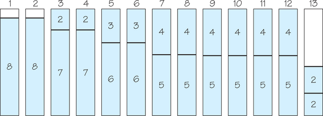
Is there any packing that uses only 12 bins? No. In Figure 3.21, there are only 2 free units (1 unit each in bins 1 and 2) of space in the first 12 bins, but 4 occupied units (two 2s) in bin 13. We could have predicted this by dividing the total length of the shelves (110) by the capacity of each bin (board): 1109=1229. Thus, no packing could squeeze these shelves into 12 bins; there would always be at least 2 units left over for the 13th bin. (In Figure 3.21, there are 4 units in bin 13 because of the 2 wasted empty spaces in bins 1 and 2.) Even if this division created a zero remainder, there would still be no guarantee that the items could be packed to fill each bin without wasted space. For example, if the bin capacity is 10 and there are weights of 6, 6, 6, 6, and 6, the total weight is 30; dividing by 10, we get 3 bins as the minimum requirement. Clearly, however, 5 bins are needed to pack the five 6s.
None of the six heuristic methods shown will necessarily find the optimal number of bins for an arbitrary problem. How can we decide which heuristic to use? One approach is to see how far from the optimal solution each method might stray.
Various formulas have been discovered to calculate the maximum discrepancy between what a bin-packing algorithm actually produces and the best possible result. For example, in situations where a large number of bins are to be packed, FF can be off by as much as 70%, but FFD is never off by more than 22%. Of course, FFD doesn’t give an answer as quickly as FF, because extra time for sorting a large collection of weights may be considerable. Also, FFD requires knowing the whole list of weights in advance, whereas FF does not. It is important to emphasize that a 22% margin of error is a worst-case figure. In many cases, FFD will perform much better. Results obtained by computer simulation indicate excellent average-case performance for this algorithm. In 2013, it was shown that if OPT (short for “optimum”) denotes the fewest bins to pack a collection of weights (scaled to lie between 0 and 1), then first fit will never need more than 1.7(OPT) bins to contain the weights. Examples needing 1.7(OPT) bins were constructed.
When solving real-world problems, we always have to look at the relationship between mathematics and the real world. Thus, first-fit decreasing usually results in fewer bins than next fit, but next fit can be used even when all the weights are not known in advance. Next fit also requires much less computer storage than first fit, because once a bin is packed, it need never be looked at again.
Fine-tuning of the conditions of the actual problem often results in better practical solutions and in interesting new mathematics as well. See Spotlight 3.2 for a discussion of some of the tools mathematicians use to verify and even extend mathematical truths by raising new mathematical problems.
Self Check 3
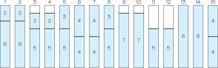
How many bins are used when you apply the first-fit bin-packing algorithm to the weights shown in Figure 3.19, using bins of size 8?
Fifteen bins are required, as shown in the accompanying diagram. A solution with fewer bins is not possible.
Using Mathematical Tools 3.2
3.2
The tools of a carpenter include the saw, T square, level, and hammer. A mathematician also requires tools of the trade. Some of these tools are the proof techniques that enable verification of mathematical truths. Another set of tools consists of strategies to sharpen or extend the mathematical truths already known. For example, suppose that if A and B hold, then C is true. What happens if only A holds? Will C still be true? Similarly, if only B holds, will C still be true?
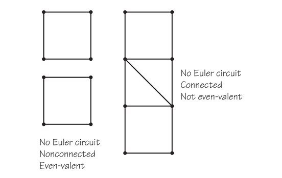
This type of thinking is of value because such questions will result either in more general cases where C holds or in examples showing that B alone and/or A alone can’t imply C. For example, we saw that if a graph G is connected (hypothesis A) and even-valent (hypothesis B), then G has a circuit that uses each edge only once (conclusion C). If either hypothesis is omitted, the conclusion fails to hold. The figures illustrate this point. on the left is an even-valent but nonconnected graph; on the right, a connected graph with two odd-valent vertices. Neither graph has an Euler circuit.
Here is another way that a mathematician might approach extending mathematical knowledge. If A and B imply C, will A and B imply both C and D, where D extends the conclusion of C? For example, not only can we prove that a connected, even-valent (hypotheses A and B) graph has an Euler circuit, but we can also show that the first edge of the Euler circuit can be chosen arbitrarily (conclusions C and D). It turns out that being able to specify the first two edges of the Euler circuit may not always be possible. Mathematicians are trained to vary the hypotheses and conclusions of results they prove, in an attempt to clarify and sharpen the range of applicability of the results.
We have seen that machine scheduling and bin packing are probably computationally difficult to solve because they are NP-complete. A mathematician could then try to find the simplest version of a bin-packing problem that would still be NP-complete: What if the items to be packed can have only eight weights? What if the weights are only 1 and 2? Asking questions like these is part of the mathematician’s craft. Such questions help to extend the domain of mathematics and hence the applications of mathematics.