4.3 4.2 Finding the Optimal Production Policy
Our next step is that we still must find the optimal production policy, a point within the feasible region that gives a maximum profit. There are a lot of points in that region. If you consider points with only whole numbers as values for x or y, there are many points, but, in fact, either x or y or both could be some fractional number. There are so many points in this feasible region that to consider the profit at each one of them would require us to calculate profits from now until we grow very old, and still the calculations would not be done. Here is where the genius of the linear-programming technique comes in, with the corner point principle, which we define in terms of our mixture problems.
Corner Point Principle THEOREM
The corner point principle states that in a linear-programming problem, the maximum value for the profit formula always corresponds to a corner point of the feasible region.
The corner point principle is probably the most important insight into the theory of linear programming. Later in this chapter, we will explain why this principle works. The geometric nature of this principle explains the value of creating a geometric model from the data in a mixture chart.
The corner point principle gives us the following method to solve a linear-programming problem:
- Determine the corner points of the feasible region.
- Evaluate the profit at each corner point of the feasible region.
- Choose the corner point with the highest profit as the production policy.
Let’s look at the feasible region that we drew in Figure 4.3 on page 133. It is a triangle having three corners; namely, (0, 0), (0, 30), and (12, 0). Now all we need to do is find out which of these three points gives us the highest value for the profit formula, which in this problem is $1.00x+$0.55y. We display our calculations in Table 4.1. The maximum profit for the toy manufacturer is $16.50, and that happens if the manufacturer makes 0 skateboards and 30 dolls. The point (0, 30) is called the optimal production policy.
| Corner Point | Value of the Profit Formula: $1.00x+$0.55y |
|---|---|
| (0, 0) | $1.00(0)+$0.55(0)=$0.00+$0.00=$0.00 |
| (0, 30) | $1.00(0)+$0.55(30)=$0.00+$16.50=$16.50 |
| (12, 0) | $1.00(12)+$0.55(0)=$12.00+$0.00=$12.00 |
Optimal Production Policy THEOREM
An optimal production policy corresponds to a corner point of the feasible region where the profit formula has a maximum value.
EXAMPLE 5![]() Finding the Optimal Production Policy
Finding the Optimal Production Policy
Our analysis of the clothing manufacturer problem resulted in a feasible region with three corner points: (0, 0), (0, 30), and (20, 0). Which of these maximizes the profit formula, $5x+$3y, and what does that corner represent in terms of how many shirts and vests to manufacture?
The evaluation of the profit formula at the corner points is shown in Table 4.2. The maximum profit of $100 occurs at the corner point (20, 0), which represents making 20 shirts and no vests.
| Corner Point | Value of the Profit Formula: $5x+$3y |
|---|---|
| (0, 0) | $5(0)+$3(0)=$0+$0=$0 |
| (0, 30) | $5(0)+$3(30)=$0+$90=$90 |
| (20, 0) | $5(20)+$3(0)=$100+$0=$100 |
General Shape of Feasible Regions
The shape of a feasible region for a linear-programming mixture problem has some important characteristics, without which the corner point principle would not work:
- The feasible region is a polygon in the first quadrant, where both x≥0 and y>0. This is because the minimum constraints require that both x and y be nonnegative.
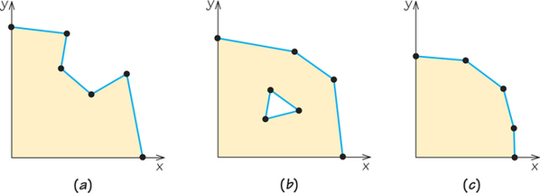
- The region is a polygon that has neither dents (as in Figure 4.5a) nor holes (as in Figure 4.5b). Figure 4.5c is a typical example. Such polygons are called convex.
The Role of the Profit Formula: Skateboards and Dolls
In practice, there are often different amounts of resources available in different time periods. The selling price for the products can also change. For example, if competition forces us to cut our selling price, the profit per unit can decrease. To maximize profit, it is usually necessary for a manufacturer to redo the mixture problem calculations whenever any of the numbers change.
Suppose that business conditions change, and now the profits per skateboard and doll are, respectively, $1.05 and $0.40. Let us keep everything else about the skateboards and dolls problem the same. The change in profits would give us a new profit formula of $1.05x+$0.40y. When we evaluate the new profit formula at the corner points, we get the results shown in Table 4.3. This time, the optimal production policy, the point that gives the maximum value for the profit formula, is the point (12, 0). To get the maximum profit of $12.60, the toy manufacturer should now make 12 skateboards and 0 dolls.
| Corner Point | Value of the Profit Formula: $1.05x+$0.40y |
|---|---|
| (0, 0) | $1.05(0)+$0.40(0)=$0.00+$0.00=$0.00 |
| (0, 30) | $1.05(0)+$0.40(30)=$0.00+$12.00=$12.00 |
| (12, 0) | $1.05(12)+$0.40(0)=$12.60+$0.00=$12.60 |
We see from this example that the shape of the feasible region, and thus the corner points we test, are determined by the constraint inequalities. The profit formula is used to choose an optimal point from among the corner points, so it is not surprising that different profit formulas might give us different optimal production policies.
We started the exploration of skateboard and doll production with the idea that a toy manufacturer has a product line with either one to two products. But both linear-programming solutions we have found tell the manufacturer that to maximize profit, make just one product. This is probably not an acceptable result for the manufacturer, who might want to produce both products for business reasons other than profit, such as establishing brand loyalty. And it certainly would be very difficult for the manufacturer to be ready to switch back and forth between producing either skateboards or dolls every time the profit formula changed. Linear programming is a flexible enough technique that it can accommodate the desire for there to be both products in the optimal production policy. This is done by specifying that there be nonzero minimum quantities for each period.
Summary of the Pictorial Method Using a Feasible Region
Let’s stop and summarize the steps we are following to find the optimal production policy in a mixture problem:
- Read the problem carefully to identify the resources and the products.
- Make a mixture chart showing the resources (associated with limited quantities), the products (associated with profits), the recipes for creating the products from the resources, the profit from each product, and the amount of each resource on hand. If the problem has nonzero minimums, include a column for those as well.
- Assign an unknown quantity, x or y, to each product. Use the mixture chart to write down the resource constraints, the minimum constraints, and the profit formula.
- Graph the line corresponding to each resource constraint and determine which side of the line is part of the feasible region. If there are nonzero minimum constraints, graph lines for them also, and determine which side of each is in the feasible region. Sketch the feasible region by finding the common points in the half-planes from all the resource constraints plus the minimum constraints. (This process is called finding the “intersection” of the half-planes.)
- Find the coordinates of all the corner points of the feasible region. Some of these may have been calculated so that you can graph the individual lines. Proceed in order around the boundary of the feasible region. Be sure that every point you consider is really a corner point of the feasible region.
- Evaluate the profit formula for each of the corner points. The production policy that maximizes profit is the one that gives the biggest value to the profit formula.
Two Products and Two Resources: Skateboards and Dolls
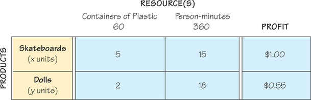
We return to the toy manufacturer now to consider two limited resources instead of one. The second limited resource will be time, the number of person-minutes available to prepare the products. Suppose that there are 360 person-minutes of labor available and that making one skateboard requires 15 person-minutes and making one doll requires 18 person-minutes. We will continue to use the original values regarding containers of plastic, the first of our two profit formulas, and to keep the problem relatively simple, we use the zero minimum constraints: x≥0 and y≥0. We need a new mixture chart. In general, we will include a column for minimums in a mixture chart only if there are any nonzero minimum constraints. In Figure 4.6, we have the mixture chart for this problem. Using the mixture chart, we can write the two resource constraints:
5x+2y≤60 for containers of plastic
and
15x+18y≤360 for person-minutes
We can also write the profit formula: $1.00x+$0.55y.

Systems of Linear Equations and Inequalities
The half-plane corresponding to the plastic resource is shown in Figure 4.7a. We now need to graph the half-plane corresponding to the time constraint. We find where the line 15x+18y=360 intersects the two axes by substituting first x=0 and then y=0 into that equation.
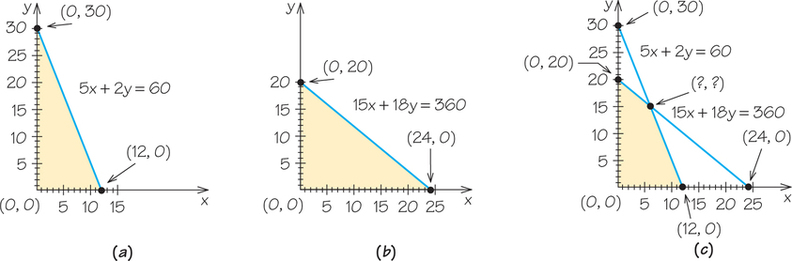
The line corresponding to the time constraint contains the two points (0, 20) and (24, 0). When we insert the point (0, 0) into the inequality 15x+18y<360, we get 15(0)+18(0)<360, or 0<360, which is true, so (0, 0) is on the side of the line that we shade. Putting all this together, we get the half-plane in Figure 4.7b as the correct half-plane for the time resource constraint.
We are not permitted to exceed the supply of even a single resource. Therefore, the feasible region must be made up of points that are shaded twice—both in the half-plane for the plastic resource constraint, shown in Figure 4.7a, and in the half-plane for the time resource constraint in Figure 4.7b. For the procedure with several half-plane constraints, we build our feasible region by finding the intersection, or overlap, of the individual half-planes in the problem. In Figure 4.7c, we show the result of intersecting the half-planes from the two resource constraints. Because this problem has minimums that are zeroes, the shaded region in Figure 4.7c is in fact the feasible region for the problem.
The next step that we need to carry out to use the pictorial method for solving this problem is to find the corner points of the feasible region. This is carried out by doing the algebra necessary to solve two linear equations in two unknowns. This leads to the points (0, 0), (0, 20), (6, 15), and (12, 0). Three of these points have a zero value for one or more of the unknowns, so the calculations are easy.
To find the coordinates of the point (6, 15), it is necessary to solve for the point that satisfies both of the equations 5x+2y=60 and 15x+18y=360. To solve these two equations simultaneously, you must multiply one or both of the equations by a number to create equivalent equations, so that when added together, one of the variables will cancel out. One way to do this is to multiply the first of these equations by −3, obtaining the equation −15x−6y=−180. When this is added to the second equation, the x term “drops out” and we can solve 12y=180, to get y=15. Now it is an easy matter to substitute this value into either of the original equations to get the x value of 6.
We are ready to finish the problem. In Table 4.4 we have evaluated the profit formula at the four corner points of the feasible region. The optimal production policy for the toy manufacturer would be to make 6 skateboards and 15 dolls, for a maximum profit of $14.25.
| Corner Point | Value of the Profit Formula: $1.00x+$0.55y |
|---|---|
| (0, 0) | $1.00(0)+$0.55(0)=$0.00+$0.00=$0.00 |
| (0, 20) | $1.00(0)+$0.55(20)=$0.00+$11.00=$11.00 |
| (6, 15) | $1.00(6)+$0.55(15)=$6.00+$8.25=$14.25 |
| (12, 0) | $1.00(12)+$0.55(0)=$12.00+$0.00=$12.00 |
Here is another mixture problem example of how the pictorial method using a feasible region works from start to finish.
EXAMPLE 6![]() Mixtures of Two Fruit Juices: Beverages
Mixtures of Two Fruit Juices: Beverages
A juice manufacturer produces and sells two fruit beverages: 1 gallon of cranapple is made from 3 quarts of cranberry juice and 1 quart of apple juice; and 1 gallon of apple-berry is made from 2 quarts of apple juice and 2 quarts of cranberry juice. The manufacturer makes a profit of 3 cents on a gallon of cranapple and 4 cents on a gallon of appleberry. Today, there are 200 quarts of cranberry juice and 100 quarts of apple juice available. How many gallons of cranapple and how many gallons of appleberry should be produced to obtain the highest profit without exceeding available supplies? We use zeroes as “reality minimums.” The mixture chart for this problem is shown in Figure 4.8.
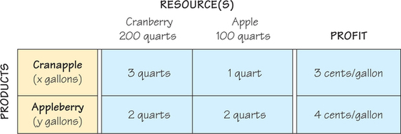
For each resource, we develop a resource constraint reflecting the fact that the manufacturer cannot use more of that resource than is available. The number of quarts of cranberry juice needed for x gallons of cranapple is 3x. Similarly, 2y quarts of cranberry are needed for making y gallons of appleberry. So if the manufacturer makes x gallons of cranapple and y gallons of appleberry, then 3x+2y quarts of cranberry juice will be used. Because there are only 200 quarts of cranberry available, we get the cranberry resource constraint 3x+2y≤200. Note that the numbers 3, 2, and 200 are all in the cranberry column. We get another resource constraint from the column for the apple juice resource: 1x+2y≤100. We also have these minimum constraints: x≥0 and y≥0.
Finally, we have the profit formula. Because 3x is the profit from making x units of cranapple and 4y is the profit from making y units of appleberry, we get the profit formula 3x+4y.
We summarize our analysis of the juice mixture problem. Maximize the profit formula, 3x+4y, given these constraints:
cranberry:3x+2y≤200apple:1x+2y≤100minimums:x≥0 and y≥0
Remember, in a mixture problem, our job is to find a production policy (x,y), that makes all the constraints true and maximizes the profit.
Figure 4.9a shows the result of graphing the constraint associated with the cranberry resource, while Figure 4.9b shows the result of graphing the constraint associated with the apple resource, taking into account that the amounts of these resources used cannot be negative. When these two diagrams are superimposed, we get the diagram in Figure 4.9c. Now, to carry out the pictorial method, we need to find the profits associated with the four corner points shown. This is done in Table 4.5.
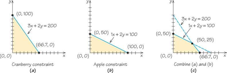
| Corner Point | Value of the Profit Formula: 3x+4y cents |
|---|---|
| (0, 0) | 3(0)+4(0)=0 cents |
| (0, 50) | 3(0)+4(50)=200 cents |
| (50, 25) | 3(50)+4(25)=250 cents |
| (66.7, 0) | 3(66.7)+4(0)=200 cents (rounded) |
When we evaluate the profit formula at the four corner points, we see that the optimal production policy is to make 50 gallons of cranapple and 25 gallons of apple- berry, for a profit of 250 cents.
Self Check 2
Maximize the profit function P=5x+3y for the feasible region associated with constraints given by the equations x≥0,y≥0,5x+2y≤60, and x≤10 (see Self Check 1 on page 134).?
- The maximal profit occurs at the feasible point (0, 30) and has value P equal to 90. The values of P at the other corner points are 0, 65, and 50.