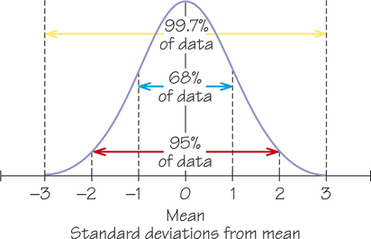
5.10 5.9 The 68-95-99.7 Rule for Normal Distributions
Because any particular normal distribution is completely determined by its mean and standard deviation, it is not surprising that all normal distributions are the same in terms of what proportion of observations are within any given number of standard deviations of the mean. Here is an important rule based on this fact.
The 68-95-99.7 Rule for Normal Distributions RULE
According to the 68-95-99.7 rule, in any normal distribution:
- About 68% of the observations fall within 1 standard deviation of the mean.
- About 95% of the observations fall within 2 standard deviations of the mean.
- About 99.7% of the observations fall within 3 standard deviations of the mean.
Figure 5.26 illustrates the 68-95-99.7 rule. By remembering these three numbers, you can think about normal distributions without making detailed calculations.
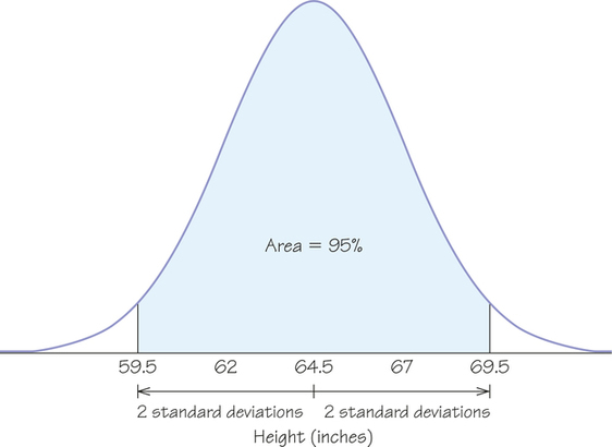
EXAMPLE 18![]() Heights of American Women: Application of the 68-95-99.7 Rule
Heights of American Women: Application of the 68-95-99.7 Rule
The heights of women between the ages of 18 and 24 are distributed roughly normally, with a mean of 64.5 inches and a standard deviation of 2.5 inches. Two standard deviations are 5 inches for this distribution. The "95" part of the 68-95-99.7 rule says that the middle 95% of young women are between 64.5−5 and 64.5+5 inches tall; that is, between 59.5 inches and 69.5 inches.
Keep in mind that this is only an approximation because the distribution of young women’s heights is approximately normal.
The other 5% of American women have heights outside the range from 59.5 to 69.5 inches. Because the normal distributions are symmetric, half of these women are on the tall side and half on the short side. So the tallest 2.5% of young women are taller than 69.5 inches.
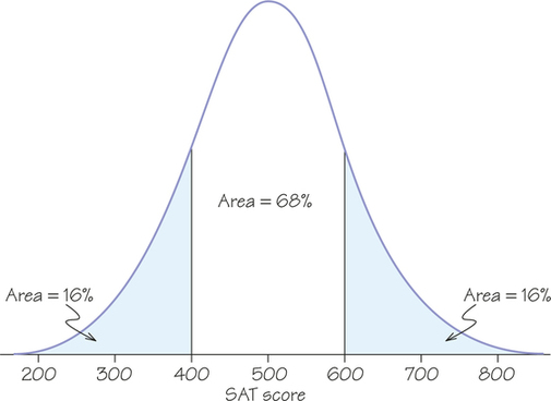
EXAMPLE 19![]() SAT Reasoning Test Scores
SAT Reasoning Test Scores
The distribution of scores on tests such as the SAT college entrance examination is close to normal. Scores on each of the three sections (math, critical reading, and writing) of the SAT are adjusted so that the mean score is about μ=500 and the standard deviation is about σ=100. (The Greek letters μ and σ designate the population mean and standard deviation, respectively, as opposed to ˉX, which designate the mean and standard deviation of sample data). This information allows us to answer many questions about SAT scores.
- How high must a student score to fall in the top 25%? This score is the 75th percentile or the third quartile. The third quartile is (0.67)(100) = 67 points above the mean. So scores above 567 are in the top 25% (i.e., the top quarter).
- What percentage of scores falls between 200 and 800? Scores of 200 and 800 are 3 standard deviations on either side of the mean—for example, 500+3×100=800. The "99.7" part of the 68-95-99.7 rule says that 99.7% of all scores lie in this interval. (In practice, the SAT makes this 100% by reporting as 200 those rare scores below 200, or as 800 those rare scores above 800.)
- What percentage of scores is above 600? A score of 600 is 1 standard deviation above the mean. By the "68" part of the 68-95-99.7 rule, 68% of all scores fall between 400 and 600 and 32% fall below 400 or above 600. Because normal curves are symmetric, half of this 32% are above 600. So a score above 600 places a student in the top 16% of test-takers. We can also say that a score of 600 is at the 84th percentile of all test-takers.
Sketching a normal curve and scaling the horizontal axis with the mean and points 1, 2, and 3 standard deviations from the mean can help you use the 68-95-99.7 rule. Figure 5.27 shows the distribution of SAT scores with the areas needed to find the percentage of scores above 600. Note that the tails of Figure 5.27, like those of any bell curve, technically stretch out forever in both directions (even as the amount of faraway area becomes vanishingly small). This is another reminder that the bell curve is a very good, but not perfect, model of reality. We know that real-life SAT subtest scores are scaled so that they do not go beyond 200 or 800.
Self Check 12
Use the distribution of SAT scores given in Example 19 to answer the following questions.
- How low must a student’s score be for it to be in the bottom 25%?
To be in the bottom 25%, a student’s score must be below the 25th percentile, which is (0.67)(100) = 67 points below the mean. So scores below 433 are in the bottom 25%.
- What percentage of the SAT scores is below 300?
A score of 300 is 2 standard deviations below the mean. Recall that 95% of observations are within 2 standard deviations of the mean, and hence, 5/2 or 2.5% are below 300.

The 68-95-99.7 rule allows you to find selected areas under a normal curve—areas for outcomes bounded by 1, 2, or 3 standard deviations away from the mean. You can use tables, software, a graphing calculator, or the Normal Density Curve applet to find any area under a normal curve. See Applet Exercises 2 to 4 to practice using the applet to find proportions.