5.8 5.7 Describing Variability: The Standard Deviation
Although the five-number summary is the most generally useful numerical description of a distribution, it is not the most common. That distinction belongs to the combination of the mean with the standard deviation. The mean, like the median, is a measure of center. The standard deviation, like the quartiles and the extremes in the five-number summary, measures variability. The standard deviation and its square, the variance, measure variability by looking at how far the observations are from their mean.
EXAMPLE 12![]() Understanding the Standard Deviation
Understanding the Standard Deviation
When you buy stocks or mutual funds, you need to be aware of how to quantify and balance mean gain with the variability or risk of the investment, especially given the volatile years the market has experienced recently. Consider the PIMCO Total Return A (symbol: PTTAX), a fund that invests in intermediate-term, fixed-income securities. Here are its annual total returns for a recent 10-year period:

| Calendar Year | 2004 | 2005 | 2006 | 2007 | 2008 | 2009 | 2010 | 2011 | 2012 | 2013 |
| Return (%) | 4.65 | 2.41 | 3.51 | 8.57 | 4.32 | 13.33 | 8.36 | 3.74 | 9.93 | −2.30 |
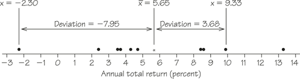
Figure 5.18 shows a dotplot of the data, with their mean (rounded to two decimals) marked by an asterisk (*). The arrows mark two of the deviations from the mean: One is positive and one is negative. We won’t get a useful measure of variability by totaling up all the positive and negative deviations because they will always sum to 0!
Squaring the deviations makes these numbers all positive, and a reasonable measure of variability is the average of the squared deviations. This average is called the variance. The variance is large if the observations are scattered widely around their mean. The variance is small if the observations are fairly close to the mean.
But the variance does not have meaningful units. With the annual return data measured in percentages, the variance of the purchase prices has units of "squared percentages." Taking the square root of the variance yields the standard deviation, which gets us back to the units of the original variable (in this case, percentages).
Self Check 7
Figure 5.18 shows the calculations for two of the deviations from the mean for the data in Table 5.8. Calculate the deviations from the mean corresponding to the other eight data values. Then verify that the sum of all 10 deviations is 0 (or close enough to 0 that any difference from 0 is due to rounding the mean to two decimals).
Here are all 10 deviations from the mean:
| −1.00 | −3.24 | −2.14 | 2.92 | −2.92 | −1.33 | 7.68 | 2.71 | −1.91 | 4.28 | −7.95 |
The sum of the deviations is 0.02, a difference from 0 that can be attributed to rounding the mean to two decimals.
Standard Deviation DEFINITION
The standard deviation is a kind of "standard" or average amount that observed data values deviate from their mean. More precisely, it is the square root of the mean of the squared deviations, except that the mean involves dividing by n−1 instead of the usual n. (It turns out n−1 makes this particular formula more accurate, but the justification is beyond the scope of this book.) In symbols, the standard deviation s of n observations x1,x2,…,xn is
s=√(x1−ˉx)2+(x2−ˉx)2+⋯+(xn−ˉx)2n−1

For simple datasets, standard deviation often can be estimated mentally by applying the first sentence of the above definition. For example, for the dataset {25, 25, 25, 30, 35, 35, 35}, we can readily see that 30 is the mean and the other numbers are each 5 units away from it. So we might assume that the standard deviation would be a value close to or equal to 5—and it is! Here are the calculations.
s=√(25−30)2 + (25−30)2 + (25−30)2 + (30−30)2 + (35−30)2 + (35−30)2 + (35−30)27−1=√25 + 25 + 25 + 0 + 25 + 25 + 256=√1506=√25=5
Even for more complex datasets, it is helpful to make a mental estimate first as a way to catch any errors caused by using a calculator. For the 10 return rate values in Example 12, a quick visual inspection might result in an estimate of the mean to be near 6 and a typical amount of deviation from 6 to be around 4, and certainly less than 8 (which is the approximate deviation of the most extreme data value from 6). Let’s keep this estimate in mind as we do the formal calculation in Example 13.
EXAMPLE 13![]() Calculating the Standard Deviation
Calculating the Standard Deviation
To find the standard deviation of the 10 return rates in Example 12, first find the mean.
ˉX=4.65+2.41+3.51+8.57+4.32+13.33+8.36+3.74+9.93+(−2.30)10=5.652%≈5.65%
For readability of Table 5.9, we have used the mean rounded to two decimals. You will get more accuracy if you include more decimal places for the mean throughout the process and do not round until the end.
| Observations | Deviations (observation minus mean) |
Squared Deviations |
|---|---|---|
| xi | xi−ˉx | (xi−ˉx)2 |
| 4.65 | 4.65−5.65=−1.00 | (−1.00)2=1.0000 |
| 2.41 | 2.41−5.65=−3.24 | (−3.24)2=10.4976 |
| 3.51 | 3.51−5.65=−2.14 | (−2.14)2=4.5796 |
| 8.57 | 8.57−5.65=2.92 | (2.92)2=8.5264 |
| 4.32 | 4.32−5.65=−1.33 | (−1.33)2=1.7689 |
| 13.33 | 13.33−5.65=7.68 | (7.68)2=58.9824 |
| 8.36 | 8.36−5.65=2.71 | (2.71)2=7.3441 |
| 3.74 | 3.74−5.65=−1.91 | (−1.91)2=3.681 |
| 9.93 | 9.93−5.65=4.28 | (4.28)2=18.3184 |
| −2.30 | −2.30−5.65=−7.95 | (−7.95)2=63.2025 |
| Sum=177.8680 | ||
The variance s2 is the sum of the squared deviations divided by 1 less than the number of observations, so it would be 177.86810−1≈19.763. The standard deviation is the square root of the variance, so we obtain s=√19.763≈4.45%. This value, 4.45%, can be considered small for this context, which suggests that this mutual fund happened to have a great deal of stability during a very turbulent decade.
Self Check 8
If the 10 observations from the fund in Example 12 still had a mean of 5.65%, but had less variability, their deviations from 5.65% would be smaller, and the standard deviation would be even smaller. To explore this dynamic, make the following changes to the data in Table 5.8: Change 13.33 to 10.33 and −2.30 to 0.7. The modified data values should have less variability because the two most extreme data values have been replaced with values closer to the mean.
- Verify that the mean of the modified data is the same as the mean of the original data from Table 5.8.
ˉx≈5.65%
- Calculate the standard deviation for the modified data. Is this value the same as, smaller than, or larger than the standard deviation of the original data?
The squared deviations for the two altered data values are (10.33−5.65)2=21.9024 and (0.7−5.65)2=24.5025. The new sum of squared deviations from the mean is 102.088. Hence, s=√102.088/9≈3.4%. This value is smaller than the standard deviation for the original data.
As you probably have noticed, calculating standard deviations using the formula given in the definition can be time consuming. In Spotlight 5.3, technology comes to the rescue!
Using Technology to Calculate Standard Deviation 5.3
5.3
While the formula in the definition box for standard deviation has conceptual clarity and a straightforward implementation (as shown in Table 5.9), it can be tedious to apply to large datasets with a basic-level calculator (such as a cell-phone calculator). Even with the most basic calculator, you’ll get the same answer faster using the following more computationally oriented formula:
s=√(x21 + x22 + ⋯ + x2n)−n(ˉx)2n−1
However, most of us have access to technology that is a bit more sophisticated than a basic-level calculator. The remainder of this spotlight is devoted to using a variety of technologies to calculate the standard deviation with a single command.
If you have a scientific calculator, put it into a STAT MODE if required, clear out any old data, and then enter your data one number at a time. (After each number, press your calculator’s data-entry button—it may say DATA or have a symbol such as [Σ or .) Once the data are entered, you can find the standard deviation by hitting the key labeled something like , or .
If you have a graphing calculator in the TI-83/84+ family (and you already used to enter one variable of quantitative data in a list, say, L1), then hit the following sequence of buttons:.
You will get not only the standard deviation (Sx), but also other descriptive statistics, including the mean and the five-number summary! Keystrokes for other specific calculator models can be found online (see the Suggested Websites for this chapter).
If your data have been entered into a column of an Excel spreadsheet, you can calculate the mean and standard deviation as follows: To calculate the mean, in an empty cell enter =AVERAGE( and then click on the first data value and drag down to the last data value. Finish the command with ) and press Enter. To calculate the standard deviation, replace =AVERAGE( with =STDEV(.
Statistical software such as JMP, Minitab, and SPSS all compute summary statistics of a dataset that include both the mean and standard deviation.
EXAMPLE 14![]() Calculating Standard Deviation Using a TI-84 Graphing Calculator
Calculating Standard Deviation Using a TI-84 Graphing Calculator
Next, we compare the fund from Example 12 (Table 5.8) with a different one—the Cohen & Steers Realty Shares (symbol: CSRSX), a mutual fund that invests in real estate investment trusts. Table 5.10 displays its calendar year total returns (in percentages) for the same 10-year period.
| 2004 | 2005 | 2006 | 2007 | 2008 | 2009 | 2010 | 2011 | 2012 | 2013 |
|---|---|---|---|---|---|---|---|---|---|
| 38.48 | 14.88 | 37.13 | −19.19 | −34.40 | 32.50 | 27.14 | 6.18 | 15.72 | 3.09 |
To calculate the mean and standard deviations for these data, we turn to a TI-84 graphing calculator.
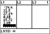
Step 1: Press (for EDIT). Enter the 10 percentages into list L1 (be sure to clear out any old data first). Here’s a screen shot after entry of the last data value:
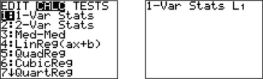
Step 2: Press and enter the command for 1-var Stats.
Step 3: Press to obtain the mean and standard deviation. Press the down arrow to obtain the five-number summary.
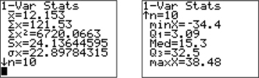
Now we are ready to compare the results for the Cohen & Steers Realty Shares (CSRSX) with the results for PIMCO Total Return A (PTTAX). On the one hand, the mean of the 10 CSRSX numbers is approximately 12.15%, which is more than double the mean from the PTTAX data. However, it comes with a tradeoff—a much higher standard deviation of approximately 24.14%. Scanning the numbers in Table 5.10, we see the dramatic lows and highs that make this fund feel like a rollercoaster ride! Knowing how to interpret these numbers is critical when making investment choices to fit your financial goals and tolerance for risk.
Self Check 9
Test grades of a sample of four students are given below. Determine the mean and standard deviation of the test grades. First, perform the calculations by applying the formulas for mean and standard deviation, and then check your results using your calculator’s (or spreadsheet’s) built-in statistical capabilities.
| Test grades: | 70 | 72 | 79 | 87 |
More important than the details of calculation of the standard deviation are the properties that determine the usefulness of the standard deviation:
- measures variability about the mean . Use to describe the variability of a distribution only when you use to describe the center.
- only when there is no variability. This happens only when all observations have the same value. (If every value is the same, every value equals the mean and thus has zero deviation from the mean!) Otherwise, . As the observations display more variability about their mean, gets larger.
- has the same units of measurement as the original observations. For example, if you measure metabolic rates in calories, both the mean and the standard deviation are also in calories.
- The use of squared deviations makes even more sensitive than to a few extreme observations. For example, dropping the Toyota Prius from our list of midsized cars drops the standard deviation of city mileages by nearly 60%, from approximately 11.10 mpg to 4.48 mpg without it. Distributions with outliers and strongly skewed distributions have large standard deviations. The number does not give much helpful information about such distributions.
We now have a choice between two descriptions of the center and variability of a distribution: (1) the five-number summary or (2) and . Because and are sensitive to extreme observations, they can be misleading when a distribution is strongly skewed or has outliers. In fact, because the two sides of a skewed distribution differ in variability, no single number such as describes the variability well. The five-number summary, with its two quartiles and two extremes, does a better job.
Although the standard deviation is widely used, it is not a natural or convenient measure of the variability of any possible distribution. The real reason for the popularity of the standard deviation is that it is the natural measure of variability for the special class of distributions called normal distributions, which we will discuss next.
Remember that a graph gives the best overall picture of a distribution. Numerical measures of center and variability report specific facts about a distribution, but they do not describe its entire shape—for example, numerical summaries do not disclose the presence of clusters. Always start with a graph of your data.
Choosing a Summary RULE
The five-number summary is usually better than the mean and standard deviation for describing a skewed distribution or a distribution with outliers. Use and only for reasonably symmetric distributions that are free of outliers.