8.3 8.2 Basic Rules of Probability
Recall from Section 8.1 that a probability model consists of two parts: the sample space and a way of assigning probabilities to events. Events are usually designated by capital letters near the beginning of the alphabet; for example, event A. The notation P(A) is shorthand for “the probability that event A will occur.” There are many ways to assign probabilities, so we will need some basic rules that any assignment of probabilities to events must obey. These rules follow from the idea of probability as “the long-run proportion of repetitions on which an event occurs.” Here are the first two rules:
- Rule 1. Any probability is a number between 0 and 1 inclusive. Any proportion is a number between 0 and 1 inclusive, so any probability is also a number between 0 and 1 inclusive. An event with probability 0 never occurs, an event with probability 1 always occurs, and an event with probability 0.5 occurs in half the trials in the long run.
- Rule 2. All possible outcomes together must have probability 1. Because some outcome must occur on every trial, the sum of the probabilities for all possible (simplest) outcomes must be exactly 1.
EXAMPLE 4![]() Assigning Probabilities to Means of Transportation
Assigning Probabilities to Means of Transportation
How do people in the United States get to work? Table 8.1 shows the results of an American Community Survey by the U.S. Census Bureau.
| Means of Travel | Frequency |
|---|---|
| Drive alone | 107,460,210 |
| Carpool | 13,675,867 |
| Public transportation (excluding taxis) | 7,053,456 |
| Walk | 3,969,058 |
| Work at home | 6,143,943 |
| Other | 2,560,426 |
| Total | 140,862,960 |
Because this is a U.S. Census Bureau survey, we can assume that the sample fairly represents the workers in the United States. Given the large sample size, the sample proportions should be good estimates of the probabilities for each category of transportation. Table 8.2 turns the data from the survey into a probability model for means of transportation to work. Notice that the probabilities are all between 0 and 1 (Rule 1) and that the sum of the probabilities is 1 (Rule 2).
| Means of Travel | Proportion/Probability |
|---|---|
| Drive alone | 0.763 |
| Carpool | 0.097 |
| Public transportation (excluding taxis) |
0.050 |
| Walk | 0.028 |
| Work at home | 0.044 |
| Other | 0.018 |
| Sum | 1 |
Based on the probabilities in Table 8.2, a randomly selected worker is almost 8 times more likely to drive alone to work than to carpool and more than 15 times more likely I to drive alone than to use pubic transportation.
When interpreting probabilities, particularly when they are small, it is helpful to make comparisons with something concrete, as we demonstrate in Spotlight 8.2.
Probability and Psychology 8.2
8.2
Our judgment of probability can be affected by psychological factors. Our desire to get rich quick may lead us to overestimate the tiny probability of winning the lottery. Our feeling that we are “in control” when we are driving may make us underestimate the probability of an accident. (This may be why some people prefer driving to flying, even though flying has a lower probability of death per miles traveled.)
The probability of winning (a share of) the 44-state Mega Millions jackpot is 1 in 258,890,850. This is less likely than picking out a particular sheet of printer paper from a stack 2.5 times the height of Mount Everest, or guessing a particular second from a period of about 8.2 years. Without concrete analogies, it is hard to grasp the meaning of very small probabilities, and some players may greatly overestimate their chances of winning, even if they buy lots of tickets. For example, suppose someone buys 20 $1 Mega Millions tickets every week for 50 years. She would have spent over $50,000, and yet her probability of winning at least one jackpot in that whole time would still be only about 1 in 5000. For comparison, the probability of dying in a car accident during a lifetime of driving is about 50 times greater than this!
Andrew Gelman, professor of statistics and political science at Columbia University, reports that most people say they would not switch to a situation in which they had a small probability p of dying and a large probability 1−p of gaining $1000. And yet, people will not necessarily spend that much for air bags for their cars. Becoming more aware of our inconsistencies and biases can help us make better use of probability when deciding what risks to take.
Sometimes it is easier to determine the probability of an event A indirectly by finding the probability of its logical opposite—that is, the event that A does not happen. The special name for this event is consistent with how the word complement is used in other contexts: the event that together with its opposite forms a complete whole—in this context, the “whole” is the entire sample space.
Complement of an Event DEFINITION
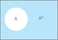
The complement of an event A is the event that A does not occur, written as Ac. (The superscript C stands for complement. Some books use the notation ˉA or A′ or “not A.”)
In the diagram in Figure 8.8, the area inside the rectangle represents the sample space. The area inside the circle represents event A, and the area inside the rectangle but outside of the circle is Ac.
For example, in the dice game of craps, rolling a sum of 7 on two dice (the most common roll) is an outcome that instantly loses the round once it’s underway. Suppose we want to know the probability of rolling anything other than a 7. If we let event A be rolling a sum of 7, then we want P(Ac), the probability of not rolling a sum of 7. The relationship between P(A) and P(Ac) is given in Rule 3, the complement rule.
- Rule 3. Complement Rule. The probability that an event does not occur is 1 minus the probability that the event does occur. Continuing the discussion above, we know from Example 3 (page 347) that the probability of rolling a sum of 7 is 16. Therefore, the probability of not rolling a sum of 7 is 1−16=56. This is really just another way of saying that the probability that an event occurs and the probability that it does not occur always add to 1, or 100% of the sample space. Referring back to the diagram in Figure 8.8, you can see how the complementary blue and white regions add up to fill the space inside the rectangle.
Another useful distinction to make when discussing two events is whether or not it is possible for the two events to happen simultaneously. If it is not possible, then the two events are said to be disjoint or mutually exclusive. An event and its complement are always mutually exclusive.
Disjoint Events (Mutually Exclusive Events) DEFINITION
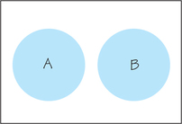
Two events are disjoint events if they have no outcomes in common. Disjoint events are also called mutually exclusive events.
In the diagram in Figure 8.9, the two circular areas represent events A and B. Since there is no overlap in these areas, the two events are disjoint.
Rule 4, the addition rule, addresses how to assign probabilities to the event that either A or B occurs in situations where events A and B are mutually exclusive.
Rule 4. Addition Rule for Disjoint Events. If two events are disjoint, the probability that one or the other occurs is the sum of their individual probabilities. Return to Example 4 (page 348). Suppose we want to determine the probability that a person drives to work either alone (event A) or in a carpool (event B). In other words, we want to determine P(A or B). From the survey data, we can calculate the number of workers who fell into events A or B: 107,460,210+13,675,867=121,136,077. So we estimate the probability from the sample proportion:
121,136,077/140,862,960≈0.860.
Instead of estimating the “long-run” proportion from the data, we can apply the addition rule for disjoint events. Simply add the corresponding probabilities from Table 8.2:
P(A or B)=P(A)+P(B)=0.763+0.097=0.860
Self Check 3
Use Table 8.2 (page 349) to determine the following probabilities:
- The probability that a randomly selected worker in the United States either uses public transportation or walks to work.
- Let A= worker uses public transportation and B= worker walks. P(A or B)=P(A)+P(B)=0.050+0.028=0.078.
- The probability that a randomly selected worker in the United States does not drive to work (either alone or in a carpool).
- Let A= worker drives to work; P(Ac)=1−P(A)=1−0.860=0.140.
Sometimes we are interested in determining the probability that either A or B occurs in cases where A and B are not disjoint. We return to the situation in which a red and green die are rolled together (for the sample space, see Figure 8.7, page 347). Consider the following events:
A=red die shows″
Suppose we want to determine ( or ). This situation is depicted by the diagram in Figure 8.10. There is an overlap in these two events: The outcome that red shows “1” and green shows “6” belongs to both and . So we can’t use Rule 4 to determine the probability that “either or occurs.” Unlike in usual everyday usage, the mathematical use of “or” is inclusive, which means that the event “ or ” happens so long as at least one of the two events happens. In set theory, this is called “the union of and ,” and it includes A’s and B’s “separate property” (the red and blue areas in the diagram) as well as their “community property” (the area where red and blue are blended). Rule 5 will provide the adjustment needed to deal with the overlap of and .
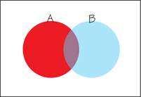
Rule 5. General Addition Rule. The probability that one event or the other occurs is the sum of their individual probabilities minus the probability of their intersection. This general addition rule makes sense if we look at Figure 8.10. Simply adding the probabilities of the two events and would overshoot the answer because we would be incorrectly counting the overlap twice. The way to adjust for this is to subtract the overlap so that it is counted exactly once. Now, we return to events and above. Their intersection corresponds to rolling “red = 1, green = 6,” which has a probability. Therefore,
We now state Rules 1 through 5 more concisely using more formal mathematical notation. As you apply these rules, remember that they are just another form of true facts about long-run proportions.
Probability Rules RULE
- Rule 1. The probability of any event satisfies .
- Rule 2. If is the sample space in a probability model, then .
- Rule 3. The complement rule: .
- Rule 4. The addition rule for disjoint events: .
- Rule 5. The general addition rule: .
In Example 5, we return to the situation of rolling two dice, which will provide an opportunity to practice applying Rules 1 through 5.
EXAMPLE 5![]() Probabilities for Rolling Two Dice
Probabilities for Rolling Two Dice
Figure 8.7 (page 347) displays the 36 possible outcomes of rolling two dice. For casino dice, it is reasonable to assign the same probability to each of the 36 outcomes in Figure 8.7. Because all 36 outcomes together must have probability 1 (Rule 2), each outcome must have probability .
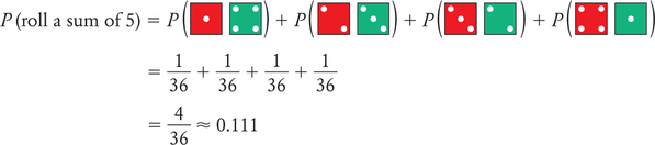
Suppose we want to determine the probability of rolling a sum of 5. Because there are four ways to roll a sum of 5, the addition rule for disjoint events (Rule 4) says that its probability is
Similarly, we can find the probabilities for the other possible sums and, in this way, get the full probability model (sample space and assignment of probabilities) for rolling two dice and summing the spots on the sides facing up. The result is shown in Table 8.3.
| Outcome (sum of two dice) | 2 | 3 | 4 | 5 | 6 | 7 | 8 | 9 | 10 | 11 | 12 |
| Probability |
The model in Table 8.3 assigns probabilities to individual outcomes. Note that Rule 2 is satisfied because all the probabilities add up to 1. To find the probability of an event, just add the probabilities of the outcomes that make up the event. For example:
Suppose we want the probability of rolling an even number. We could find this probability by finding the sum of the following:
But a faster way would be to use the complement rule (Rule 3):
For an example of Rule 5, let event be “sum is odd” and event be “sum is a multiple of 3.” Suppose we want . Earlier, we calculated . You can verify that and . Now we are ready to apply Rule 5:
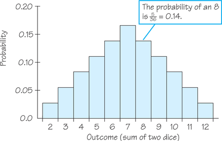
When the outcomes for a probability model are numbers, such as for the model in Table 8.3, we can use a histogram to display the assignment of probabilities to the outcomes. Figure 8.11 is a probability histogram of the probability model in Table 8.3. The height of each bar shows the probability of the outcome at the base of the bar. Because the heights are probabilities, they add to 1. Think of Figure 8.11 as an idealized picture of the results of very many rolls of a pair of dice. As an idealized picture, it is perfectly symmetric about the middle bar corresponding to a sum of 7.