Algebra Review IV: Linear Equations and Inequalities
A. Linear equations in one Variable
A linear equation in one variable is an equation that involves only the first power of the variable (typically represented by x) and no division by any expression involving the variable. Here are some examples of linear and nonlinear equations.
Linear EquationsNonlinear Equations2x=6x2+1=60.3(w−5)+4=6.1+0.1w3x+4=512(x+2)=37(2x−1)=4√p(1−p)25=0.1
A linear equation can be solved by performing the following steps:
- Simplify both sides of the equation. This includes removing all parentheses and combining all like terms. If the equation has fractions, clearing these will generally simplify the remaining steps. To clear the fractions, multiply both sides of the equation by a number divisible by all denominators of the fractions.
- Place all terms involving the variable on one side of the equation; place everything else on the other side of the equation.
- Combine like terms or factor the variable out of all terms.
- Divide both sides by the coefficient of the variable.
Not every equation will require all four steps.
Example 1. Solve 12(x+2)+37(2x−1)=4 for x.
STEP 1. Simplify both sides of the equation.
12(x+2)+37(2x−1)=4Clear the fractions:Multiply both sidesof the equation by 14,the smallest numberdivisible by both 2and 7.14(12(x+2)+37(2x−1))=14(4)Multiply each term on theleft-hand side by 14.(Use the distributive law.)14(12(x+2))+14(37(2x−1))=14[4]Perform the multiplicationsby 14.7(x+2)+6(2x−1)=56Apply the distributivelaw to remove the parentheses.7x+14+12x−6=56Simplify by combiningterms involving x andconstant terms.19x+8=56
STEP 2. There is only one term involving x, which is on the left-hand side. Place all terms not involving x to the right-hand side of the equation.
19x+8=56Subtract 8 from both sidesof the equation.19x+8−8=56−8
STEP 3. Combine like terms.
19x=48
STEP 4. Solve for x.
19x19=4819Divide both sides of theequation by 19, thecoefficient of x.x=4819
Example 2. Solve 0.3(w−5)+4=6.1+0.1w for w.
STEP 1. Simplify both sides of the equation.
0.3(w−5)+4=6.1+0.1wRemove parentheses onthe left-hand side bymultiplication.0.3w−1.5+4=6.1+0.1wCombine the constantterms on the left-hand side.0.3w+2.5=6.1+0.1w
STEP 2. Place all terms with w on the left side of the equation and all other terms on the right side.
−0.3w+2.5=6.1+0.1wAdd −0.1w−2.5 to bothsides of the equation.0.3w+2.5−|0.1w−2.5=6.1+0.1w−0.1w−2.5
STEP 3. Combine like terms.
0.2w=3.6
STEP 4. Solve for w.
0.2w0.2=3.60.2Divide both sides of theequation by the coefficient of w.w=18
Practice Exercises
Solve the following equations for x.
- 2x=6
- 40−2x=19+5x
- 2.8−2(x−1.3)=1.6x
- 23x−6=4−12x
- 4(1−5x)=2(x−1)+6x
- 1−4(2x)=6−(x+6)
- 15(2−x)+1=110x
- 14x+12(x−4)=3−16(x−2)
B. Plotting Points in the Plane
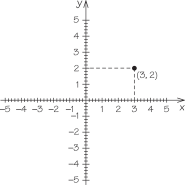
To form a coordinate plane, place two number lines at right angles, so they cross at 0. The number lines are called axes. Usually, the horizontal axis is labeled as the x-axis and the vertical axis is labeled as the y-axis. A point in the coordinate plane is specified by an ordered pair (x, y). To plot an ordered pair, such as (3, 2), draw a vertical line through the x-axis at x=3 and a horizontal line through the y-axisat y=2. The point of intersection of these two lines is the point (3, 2).
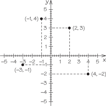
Example 1. Plot the points (2, 3), (−1, 4), (4, −2), and (−3,−1).
Practice Exercises
- Plot the points (1, 3), (1, −2), (1, 1), and (1, −4). What pattern do you notice about these points?
- Plot the points (2, −2), (4, −2), (−2, −2), and (1, −2). What pattern do you notice about these points?
- Plot the points (−4, −4), (−2, −2), (0, 0), (1, 1), and (3, 3). What pattern do you notice about these points?
C. Distance and Midpoint between Two Points in the Plane
Given two points in the plane, sometimes we will want to calculate the distance between them; other times, we will want to place a point midway between the two points. Given two points in the plane, (x1,y1) and (x2,y2), we use the following formula to find the distance between them.
Distance between (x1,y1) and (x2,y2):
D=√(x2−x1)2+(y2−y1)2
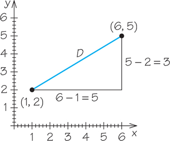
Example 1. Find the distance between the points (1, 2) and (6, 5).
D=√(6−1)2+(5−2)2=√52+32=√25+9=√34≈5.83
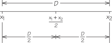
To find the midpoint between two numbers on a number line, simply average the two numbers.
Midpoint between x1 and x2: Midpoint x1+x22
Example 2. Determine the midpoint between 2 and 12.
The distance between 2 and 12 is 10. So the midpoint should be 102, or 5, units from both 2 and 12. Using the midpoint formula we get:
Midpoint=2+122=172=7
Notice that 7 is 5 units above 2 and 5 units below 12.
We can also find the midpoint of a line segment between two points (x1,y1) and (x2,y2). The x- and y-coordinates of the midpoint will be the average of the x- and y-coordinates of the two points, respectively.
Midpoint between (x1,y1) and (x2,y2) is
(x1+x22,y1+y22)
Example 3. Find the midpoint between the points (1, 2) and (6, 5). Then find the distance between (1, 2) and the midpoint and the distance between the midpoint and (6, 5). What is true of these two distances?
Midpoint=(1+62,2+52)=(72,72)
The distance between (1, 2) and (72,72) is
D=√(72−1)2+(72−2)2=√(52)2+(32)2=√344=√342
The distance between (72,72) and (6, 5) is
D=√(1−72)2+(5−72)2=√(52)2+(32)2=√344=√342
These two distances are equal, half the distance between (1, 2) and (6, 5).
Practice Exercises
- Find the distance between (2, 1) and (7, 10).
- (a) Find the midpoint of the line segment between (2, 1) and (7, 10).
- (b) Use the distance formula to find the distance between (2, 1) and the midpoint from part (a), as well as the distance between the midpoint and (7, 10). What is true of these two distances?
- (a) Find the distance between (−2,−7) and (3, 4).
- (b) Determine the midpoint of the line segment between (−2,−7) and (3, 4).
- (a) Find the distance between (−6,−7) and (1, −3).
- (b) Determine the midpoint of the line segment between (−6,−7) and (1, −3).
D. Linear equations in TWO Variables
A linear equation in two variables (typically x and y) can be written in the form ax+by=c. A solution to such an equation is an ordered pair, (x, y), that satisfies the equation.
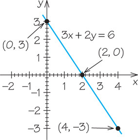
Example 1. Verify that (4, −3) is a solution to 3x+2y=6.
Substitute 4 for x and −3 for y, and then simplify to show that the expression on the left side of the equation is equal to 6, the number on the right side.
3(4)+2(−3)?=612+(−6)?=66=6 True
Example 2. Show that (1, 1) is not a solution to 3x+2y=6.
3(1)+2(1)?=63+(2)?=65=6 True
A line is a visual representation of the linear equation’s solution set and can be graphed by drawing a line through two distinct points in the solution set. When the linear equation is in the form ax+by=c, an efficient method of graphing is to graph by intercepts. The y-intercept can be found by substituting x=0 and then solving for y. The x-intercept can be found by substituting y=0 and then solving for x. To graph ax+by=c, draw a line through the x- and y-intercepts.
Example 3. Determine the x and y intercepts for 3x+2y=6. Draw a line that represents the solution set.
To find the y-intercept, substitute x=0 and solve for y:
3(0)+2y=60+2y=62y=6y=3
The y-intercept is the ordered pair (0, 3).
To find the x-intercept, substitute y=0 and solve for x:
3x+2(0)=63x+0=63x=6x=2
The x-intercept is the ordered pair (2, 0).
To graph 3x+2y=6, plot the two intercepts and then draw a line through them as shown below. Notice that (4, −3) (see Example 1) is on the line, but (1, 1) (see Example 2) is not.
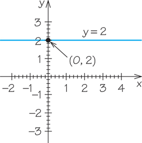
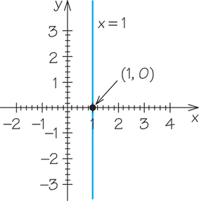
Two special kinds of lines of interest are horizontal and vertical lines. A horizontal line can be written in the form y=b (b is where the line crosses the y-axis). A vertical line can be written in the form x=a (a is where the line crosses the x-axis).
Example 4. Graph the solution set of 4x+6y=4(3+x).
Start by simplifying the equation and getting all variables to one side of the equation.
4x+6y=4(3+x)Remove the parenthesesby multiplying. (Use thedistributive law.)4x+6y=12+4xSubtract 4x from both sides of theequation.6y=12Divide both sides of the equationby 6, the coefficient of y.y=2
The graph of the solution set is a horizontal line with y-inter- cept at (0, 2).
Example 5. Graph the line x=1.
The graph is a vertical line with x-intercept (1, 0)
Practice Exercises
- Is (3, 4) a solution to 4x+3y=10?
- Is (1, 2) a solution to 4x+3y=10?
- Find the x- and y-intercepts for 4x+3y=10. Draw a line that represents the solution set.
- Express 4x−5y=2(3+x) in the form ax+by=c.
- Is (2,−25) a solution to the linear equation in Practice Exercise 4?
- Find the x- and y-intercepts for the linear equation in Practice Exercise 4. Draw a line that represents the solution set.
- Graph the solution set of 6x+4y=4(2+y).
- Graph the solution set of 14x+2y=2(5x−3)+4x.
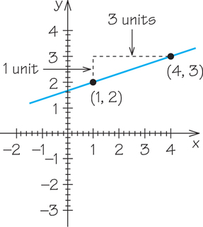
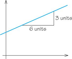
E. slope of a Line
The slope of a line is defined to be the ratio of the vertical change to the horizontal change. If we think of slope as m=change in ychange in x′, the slope of the line below would be m=13.
Given two points (x1,y1) and (x2,y2), the formula to calculate slope is m=y2−y1x2−x1.
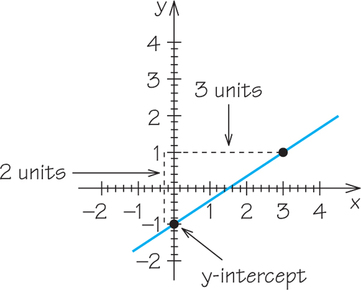
Example 1. Calculate the slope of a line that passes through the points (1, 3) and (4, 0).
By letting (x1,y1)=(1,3) and (x2,y2)=(4,0), the slope of the line below would be m=y2−y1x2−x1=0−34−1=−33=−1
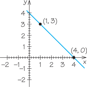
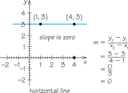
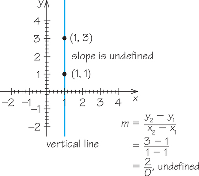
Given a graph of a line, we can determine visually whether the slope is positive or negative. If the y-values increase as the x-values increase, as is the case in the graph that appears before Example 1, then the slope is positive. On the other hand, if the y-values decrease as the x-values increase, as is the case for the graph in Example 1, then the slope is negative. Horizontal lines have a slope of 0. Vertical lines have undefined slope.
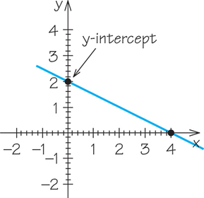
Example 2. Graph the line that passes through the points (1, 3) and (4, 3). Determine its slope.
Example 3. Graph the line that passes through the points (1, 3) and (1, 1). Determine its slope.
(For additional help in computing slopes, see Example 2 in Algebra Review III, item A, Using Formulas, page AR-7.)
Practice Exercises
For Practice Exercises 1–4, determine the slope of the line that passes through the given points.
- 1. (5, 1) and (20, 6)
- 2. (4, −2) and (8, −6)
- 3. (5, −2) and (5, 2)
- 4. (−3,8) and (−5,8)
- 5-8. Determine whether the slope of each line in the graph below is positive, negative, zero, or undefined.
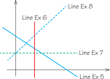
- 9. Determine the slope of the line given the information in the graph below.
F. Graphing a Line in slope-Intercept Form
When a linear equation is written in the form y=mx+b, it is said to be in slope-intercept form. In this form, b is the location where its graph intersects the vertical axis, which is generally referred to as the y-intercept. This intercept represents one point on the graph of the line. In order to graph a line, two points are required. A second point can be obtained by using the slope.
Example 1. Graph the line y=23x−1 by first plotting the y-intercept and then using the slope to find a second point on the line.
In the graph below, first plot the y-intercept, (0,−1). Using the slope of 23, find a second point on the line by starting at (0,−1) moving up 2 units and to the right 3 units, which gives the point (3, 1). Draw a line through (0,−1) and (3, 1).
Example 2. Graph the line y=−0.5x+2.
First, plot the y-intercept, (0, 2). Instead of using the slope to obtain a second point, it may be easier to evaluate the formula with a value for x other than x=0. For example, if we substitute x=4, we find that y=−0.5(4)+2=−2+2=0. This corresponds to the point (4, 0). By drawing a line through the y-intercept and the point (4, 0), we have the following graph:
Calculator Note: You can use a graphing calculator to graph a line in the form y=mx+b. Here’s how:
- Press Y=. Clear out any stored functions.
- Enter the function, mx+b, as Y1 and then press ZOOM6 to graph the line in the standard viewing window (Xmin]).
- If needed, press WINDOW and adjust the scaling.
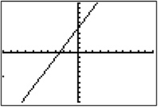
Example 3. Using a graphing calculator, graph in the standard viewing window.
Following the note above, enter opposite Y1. Your graph should be similar to the screenshot shown below.
Practice Exercises
- A line crosses the -axis at 4 and has slope . Write an equation that describes the line.
- A line has -intercept of (0, ) and slope of 2. Identify a second point on the line.
- A line is described by the equation . Starting at the -intercept, use the slope to plot a second point that lies on the line that has an -coordinate equal to 4. Draw a line through the -intercept and second point.
- Plot two points on the line described by . Draw a graph of the line. (You may have to extend your horizontal axis in order to see where your graph crosses the -axis.)
- (a) The points (2, 5) and (4, 9) lie on a line. What is the slope of the line?
- (b) Substitute the slope into the equation . Substitute one of the points and solve for .
- (c) Finally, write an equation that describes the line through the points (2, 5) and (4, 9).
- Repeat Practice Exercise 5 using the points (1, 7) and (3, 2).
For Practice Exercises 7 and 8, use a graphing calculator to graph the equations.
- . (Adjust the window settings: .)
G. Linear Inequalities in TWO Variables
To graph linear inequalities, we first graph the line, determine whether the line should be drawn solid or dashed, and then determine which side of the line to shade.
- We draw a solid line in cases where the points on the line are included in the solution set (the inequality is inclusive, or ) and a dashed line when the points on the line are not part of the solution set (the inequality is not inclusive, or ).
- To determine which side of the line to shade, we substitute a test point. A test point can be any point in the plane that is not on the line. In most cases, choosing the origin as a test point allows for easy calculation. If substituting the test point results in an inequality that is true, shade the region on the side of the line containing the test point; otherwise, shade the region on the opposite side of the line to the test point.
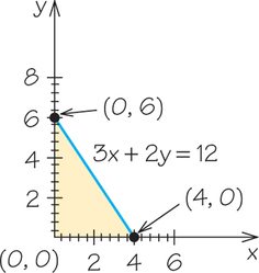
Example 1. Graph in the first quadrant.
This line has a -intercept of (0, 6) and an -intercept of (4,0). We draw a solid line because of the inclusive inequality symbol , which indicates that the points on the line are part of the solution. Next, we test to see if (0, 0) is in the solution set: , or , is a true statement. Therefore, we shade the region on the side of the line containing our test point.
Calculator Note: To graph a linear inequality, you will first need to solve the inequality for . In other words, express the inequality in the form , where the inequality sign could be any of the four possibilities: .
The following algebraic manipulations do not change the solution set of an inequality:
- Adding or subtracting the same quantity to both sides of the inequality.
- Multiplying or dividing both sides of the inequality by the same positive quantity.
- Multiplying or dividing both sides of the inequality by the same negative number and reversing the direction of the inequality sign.
Example 2. Use a graphing calculator to graph .
STEP 1. Solve the inequality for .
- STEP 2. Using the test point (0, 0), we find that , which is a true statement. The solution set is the region on the side of the line containing (0, 0).
STEP 3. Enter the linear function into your calculator’s function list.
- Press and clear any stored functions.
- Enter the function as Y1. Press and then to graph the line in the standard viewing window.
- The test point (0, 0) lies below the line. So next we shade that region. Press . The cursor should be to the right ofY1. Use the left arrow key to move the cursor to the left of Y1. Press repeatedly until the “shade below” symbol is displayed. Press . The result appears below.
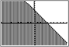
Unlike in Example 1, for Example 2 we did not restrict the solution set to the first quadrant.
Note: You will need to determine whether to draw a solid line or a dotted line. In this case, a solid line should be drawn because of the inclusive inequality .
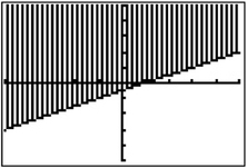
Example 3. Use algebraic manipulation to solve the following inequality for . Use a graphing calculator to graph the solution set.
STEP 1. Solve the inequality for .
Page AR-17- STEP 2. Using the test point (0, 0), we find , which is true. So, we will shade the side of the line that contains the test point.
STEP 3. Graph , determine which side of the line to shade and then graph the solution set. The result appears below. The viewing window is set so that the values for and are between and 5. The region above the line is shaded because the test point (0, 0) lies above the line.
Practice Exercises
- Does (1, 3) belong to the solution set of ?
- Does (4, 2) belong to the solution set of ?
Graph the solution set of as follows:
- (a) Graph . (Should you draw this line solid or dashed?)
- (b) Select a test point. Does your test point make the inequality true or false?
- (c) Shade the region corresponding to the solution set.
- Graph the solution set of . Use the test point from Practice Exercise 1 to determine which region should be shaded. (If this test point does not help, select a different test point.)
- 5. Graph the solution set of . Use the test point from Practice Exercise 2 to determine which region should be shaded. (If this test point does not help, select a different test point.)
- Solve for . [In other words, express in the form .]
- Use a graphing calculator to graph the solution set of . Make a sketch of the graph.
- Use a graphing calculator to graph the solution set of . Make a sketch of the graph.
H. systems of Linear Equations and Inequalities
Systems of Linear Equations
Two or more linear equations that are to hold true at the same time are called a system of linear equations. Systems of linear equations can be represented by graphing the linear equations and determining the point of intersection, if one exists. The point of intersection is the solution to the system of linear equations.
Here is a general strategy for solving a system of two equations in two variables:
- STEP 1. Solve one of the equations for one of the variables. Substitute this expression into the second equation to obtain one equation in one variable.
- STEP 2. Solve this new equation using the techniques from Part IV, item A, Linear Equations in One Variable (page AR-10).
- STEP 3. Use the solution from Step 2 and either of the original equations to compute the corresponding value for the second variable.
Example 1. Solve the system:
STEP 1. Solve equation (1) for and then substitute the expression for into equation (2).
STEP 2. Solve the equation from Step 1 for .
STEP 3. Find the corresponding value for by substituting 3 for in either equation (1) or (2).
The solution is (3, 2).
Finally, we check that our solution is correct:
Example 2. Represent graphically the system of equations from Example 1.
We can use the graph-by-intercept approach (see Algebra Review IV, item D, Linear Equations in Two Variables, page AR-13) to graph the two linear equations. Below are graphs of equations (1) and (2), along with their corresponding x- and y-intercepts. The solution to the system of equations is the point of intersection of the two lines, which appears to be (3, 2).
Calculator Note: Next, we find the solution to the system of linear equations in Example 1 using a TI-84 graphing calculator.
First we solve equations (1) and (2) for , which results in the following equations:
Next, use a TI-84 graphing calculator to graph equations and :
- Press , clear any previously stored functions, and enter the expressions for and as functions Y1 and Y2, respectively.
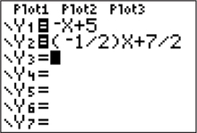
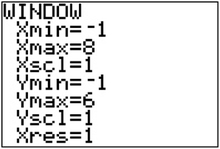
- Press and adjust the window settings to .
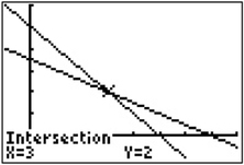
Now you need to find the point of intersection. Here’s how:
- Press (for CALC) (for intersect).
- Press twice in response to “First curve?” and “Second curve?”.
- Use the arrow keys to move the cursor close to the point of intersection and press .
- Read off the solution or (3, 2) as shown in the screenshot.
Systems of Linear Inequalities
If you are given more than one inequality, then you have a system of linear inequalities. In graphing a system of linear inequalities, you look for the region that is common to the graphs of all the individual inequalities.
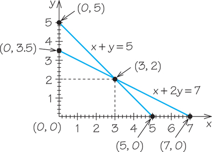
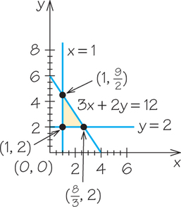
Example 3. Graph the solution set of .
Begin by graphing the equations . We have drawn solid lines in the graph that follows because each of the inequalities is inclusive ( or ). We can see that the shaded region satisfies all three inequalities. In addition, the three points of intersection are shown. These were found by examining the three lines two at a time.
Calculator Note: Since is not a function (it fails the vertical line test), you cannot graph it using the menu on a TI-84 graphing calculator. Graph the other functions first and approximate the graph of by pressing (for DRAW) and then (for Vertical), followed by . Use the left or right arrow keys to move the vertical line as close as possible to its desired location. (You won’t be able to get it exact.)
Practice Exercises
Check to see if (4, 1) is a solution to the system of equations
For Practice Exercises 2 and 3, use algebraic procedures to solve the system of equations.
(a) Use algebraic procedures to solve the following system of equations:
- (b) What problem did you encounter?
- (c) Graph the system of equations, and explain why this system has no solution.
Use a graphing calculator to solve the following system of equations:
- Check whether (1, 3) is in the solution set to .
- Graph the solution set of .
- Graph the solution set of .