1 International Trade Agreements
1. Objectives:
a. Explain the logic of multilateral agreements (like the WTO). The analysis will assume two large countries, but this is not restrictive since the most favored nation principle guarantees that all tariff reductions in the WTO apply to all members.
b. Discuss regional trade agreements and their relation to multilateral agreements.
2. The Logic of Multilateral Trade Agreements
a. Tariffs for a Large Country
Review how a tariff by a large country gives it a TOT gain, but that this is mirrored by a TOT loss for the other country.
b. Payoff Matrix
Now allow for strategic interaction between the two countries. Use a 2x2 payoff matrix with “no tariff” and “tariff” as the strategies and welfare changes relative to free trade as payoffs. Assume symmetry.
c. Free Trade
If neither country imposes a tariff there is no welfare loss, so the payoff to each is zero.
d. Tariffs
If one country imposes a tariff it gains, but the other country takes a large loss. If both countries impose a tariff, they both lose.
e. Prisoner’s Dilemma
Note that this is a prisoner’s dilemma game.
f. Nash Equilibrium
Explain that the unique Nash equilibrium is for both countries to impose tariffs.
g. Trade Agreement
A trade agreement commits both countries to free trade, so that both are better off.
3. Regional Trade Agreements
Regional trade agreements are common and permitted by WTO. However, they contradict the most favored nation principle because members get preferential treatment over nonmembers. Types:
a. Free-Trade Area
A free-trade area eliminates trade barriers between members, but keeps existing barriers with the rest of the world. Example: NAFTA.
b. Customs Union
Like a free-trade area except that it imposes a common trade policy. Example: EU.
c. Rules of Origin
Free-trade areas implement “rules of origin,” that preclude nonmembers from “arbitraging” differences in tariff rates between member countries. This is not needed in a customs union.
4. Trade Creation and Trade Diversion
Regional trade agreements increase trade in two ways: (1) Trade creation, when a country imports goods from other member countries that it formerly produced itself (like the gains from trade in H-O or Ricardian theory); (2) trade diversion, when a country imports a good from another member that it formerly imported from nonmembers.
5. Numerical Example of Trade Creation and Diversion
A numerical example estimating the trade diversion (between the U.S. and China) and trade creation (between the U.S. and Mexico) in the market for auto parts caused by NAFTA.
6. Trade Diversion in a Graph
Draw export supply and import demand for auto parts, with supply coming from Mexico and China with both facing a common U.S. tariff. Now allow Mexico to be duty free. Calculate welfare effects on the U.S. and Mexico: Mexico gains producer surplus, but U.S. loses tariff revenue, so joint welfare actually decreases.
a. Interpretation of the Loss
China is the most efficient producer of parts, so diverting production to Mexico raises MC. Paradoxically, the loss comes from eliminating a tariff, rather than imposing one.
b. Not All Trade Diversion Creates a Loss
This perverse result need not occur. Suppose that, after joining NAFTA, Mexican productivity increases due to investment. Mexican MC will fall, so it will fully replace China as the supplier to the U.S.
When countries seek to reduce trade barriers between themselves, they enter into a trade agreement—a pact to reduce or eliminate trade restrictions. Multilateral trade agreements occur among a large set of countries, such as the members of the WTO, that have negotiated many “rounds” of trade agreements. Under the most favored nation principle of the WTO, the lower tariffs agreed to in multilateral negotiations must be extended equally to all WTO members (see Article I in Side Bar: Key Provisions of the GATT, in Chapter 8). Countries joining the WTO enjoy the low tariffs extended to all member countries but must also agree to lower their own tariffs.
The WTO is an example of a multilateral trade agreement, which we analyze first in this section. To demonstrate the logic of multilateral agreements, we assume for simplicity that there are only two countries in the world that enter into an agreement; however, the theoretical results that we obtain also apply when there are many countries. The important feature of multilateral agreements is that no countries are left out of the agreement.
Following our discussion of multilateral agreements, we analyze regional trade agreements that occur between smaller groups of countries and find that the implications of regional trade agreements differ from those of multilateral trade agreements. When entering into a regional trade agreement, countries agree to eliminate tariffs between themselves but do not reduce tariffs against the countries left out of the agreement. For example, the United States has many regional trade agreements, including those with Israel, Jordan, Chile, with the countries of Central America and the Dominican Republic (through an agreement called CAFTA-DR), and new agreements being planned with South Korea, Panama, and Colombia, which have not been ratified.2 In South America, the countries of Argentina, Brazil, Paraguay, Uruguay, and Venezuela belong to a free-trade area called Mercosur. In fact, there are more than 200 free-trade agreements worldwide, which some economists feel threaten the WTO as the major forum for multilateral trade liberalization.
The Logic of Multilateral Trade Agreements
Before we begin our analysis of the effects of multilateral trade agreements, let’s review the effects of tariffs imposed by large countries under perfect competition.
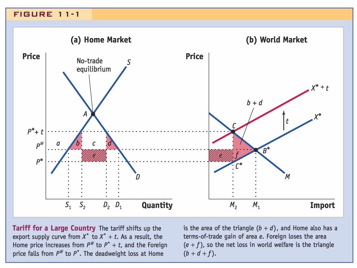
Tariffs for a Large Country In Figure 11-1, we show the effects of a large-country (Home) tariff, repeated from an earlier chapter. We previously found that a tariff leads to a deadweight loss for Home, which is the sum of consumption and production losses, of area (b + d) in Figure 11-1. In addition, the tariff leads to a terms-of-trade gain for Home, which is area e, equal to the reduction in Foreign price due to the tariff, (PW − P*), multiplied by the amount of Home imports under the tariff, (D2 − S2). If Home applies an optimal tariff, then its terms-of-trade gain exceeds its deadweight loss, so that e > (b + d). Panel (b) shows that for the rest of the world (which in our two-country case is just Foreign), the tariff leads to a deadweight loss f from producing an inefficiently low level of exports relative to free trade, and a terms-of-trade loss e due to the reduction in its export prices. That is, the Home terms-of-trade gain comes at the expense of an equal terms-of-trade loss e for Foreign, plus a Foreign deadweight loss f.
Reviewing the optimal tariff argument is important to set the stage here, but emphasize that for our story to work the tariff need not be "optimal." There is a range of small tariffs that yield e > b + d.
371
Payoff Matrix This quick review of the welfare effects of a large-country tariff under perfect competition can be used to derive some new results. Although our earlier analysis indicated that it is optimal for large countries to impose small positive tariffs, that rationale ignored the strategic interaction among multiple large countries. If every country imposes even a small positive tariff, is it still optimal behavior for each country individually? We can use game theory to model the strategic choice of whether to apply a tariff, and use a payoff matrix to determine the Nash equilibrium outcome for each country’s tariff level. A Nash equilibrium occurs when each player is taking the action that is the best response to the action of the other player (i.e., yielding the highest payoff).
372
In Figure 11-2, we show a payoff matrix between the Home and Foreign countries (both large), each of which has to decide whether to impose a tariff against the other country. Each quadrant of the matrix includes Home’s payoff in the lower-left corner and Foreign’s payoff in the upper-right corner. We will start with a situation of free trade and then measure the change in welfare for Home or Foreign by applying a tariff. For convenience, we will also assume that the two countries are exactly the same size, so their payoffs are symmetric.
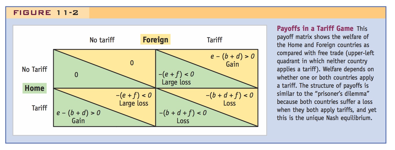
Free Trade When both countries do not impose tariffs, we are in a free-trade situation, shown in the upper-left quadrant. For convenience, let us write the payoffs for the two countries under free trade as zero, which means that we will measure the payoffs in any other situation as relative to free trade.
Tariffs First, suppose that Home imposes a tariff but Foreign does not. Then the Home payoff as compared with free trade is e − (b + d) (which is positive for an optimal tariff), and the Foreign payoff is −(e + f), the terms-of-trade and deadweight losses described previously. These payoffs are shown in the lower-left quadrant of the matrix. Now suppose that Foreign imposes a tariff but Home does not. Because we have assumed that the Home and Foreign countries are the same size, they have the same potential payoffs from using a tariff. Under these circumstances, the Foreign payoff from its own tariff is e − (b + d) > 0, and the Home payoff is the loss −(e + f). These two payoffs are shown in the upper-right quadrant of the matrix.
Finally, suppose that both countries impose optimal tariffs and that the tariffs are the same size. Then the terms-of-trade gain that each country gets from its own tariff is canceled out by the terms-of-trade loss it suffers because of the other country’s tariff. In that case, neither country gets any terms-of-trade gain but both countries still suffer a deadweight loss. That deadweight loss is (b + d) from each country’s own tariffs plus area f, the deadweight loss from the other country’s tariff. The total deadweight loss for each country is −(b + d + f), as shown in the lower-right quadrant of the matrix.
Prisoner’s Dilemma The pattern of payoffs in Figure 11-2 has a special structure called the prisoner’s dilemma. The “prisoner’s dilemma” refers to a game in which two accomplices are caught for a crime that they committed, and each has to decide whether to confess. They are kept in separate cells, so they cannot communicate with each other. If one confesses and the other does not, then the person confessing will get a much lighter jail sentence and is better off than taking the chance of being found guilty in a trial. But if they both confess, then they both go to jail for the full sentence. This is like the pattern in Figure 11-2, in which each country acting on its own has an incentive to apply a tariff, but if they both apply tariffs, they will both be worse off.
373
Work carefully through the proof of a unique Nash equilibrium. Many of the students will have encountered the prisoner's dilemma in other classes, but they probably won't know the details of the argument.
Nash Equilibrium The only Nash equilibrium in Figure 11-2 is for both countries to apply a tariff (lower-right quadrant). Starting at that point, if either country eliminates its tariff, then it loses (e + f) as compared with free trade, rather than (b + d + f). Because we know that e > (b + d) for an optimal tariff, it follows that each country acting on its own is worse off by moving to free trade (i.e., removing its tariff). That is, the loss (e + f) is greater than the loss (b + d + f). As a result, the Nash equilibrium is for both countries to apply a tariff.
Some students may have even encountered the prisoner's dilemma in a repeated game. In that case one might interpret the WTO's provision for retaliatory tariffs as a kind of trigger strategy.
But, like having both prisoners confess, the outcome for both countries when each country applies a tariff is bad. They both suffer the deadweight losses that arise from their own tariff and their partner’s tariff, without any terms-of-trade gain. The Nash equilibrium in this case leads to an outcome that is undesirable for both countries even though it is the best outcome for each country given that the other country is imposing a tariff.
Emphasize the role of the WTO as a commitment mechanism.
Trade Agreement This bad outcome can be avoided if the countries enter into some kind of trade agreement. In an earlier chapter, for example, we saw how the WTO dispute-settlement mechanism came into play when the steel tariffs applied by President Bush became problematic for the United States’ trading partners. The European Union (EU) filed a case at the WTO objecting to these tariffs, and it was ruled that the tariffs did not meet the criterion for a safeguard tariff. As a result, the WTO ruled that European countries could retaliate by imposing tariffs of their own against U.S. exports. The threat of these tariffs led President Bush to eliminate the steel tariffs ahead of schedule, and the outcome moved from both countries potentially applying tariffs to both countries having zero tariffs.
Thus, the WTO mechanism eliminated the prisoner’s dilemma by providing an incentive to remove tariffs; the outcome was in the preferred upper-left quadrant of the payoff matrix in Figure 11-2, rather than the original Nash equilibrium in the lower-right quadrant. The same logic comes into play when countries agree to join the WTO. They are required to reduce their own tariffs, but in return, they are also assured of receiving lower tariffs from other WTO members. That assurance enables countries to mutually reduce their tariffs and move closer to free trade.
Regional Trade Agreements
Under regional trade agreements, several countries eliminate tariffs among themselves but maintain tariffs against countries outside the region. Such regional trade agreements are permitted under Article XXIV of the GATT (see Side Bar: Key Provisions of the GATT, in Chapter 8). That article states that countries can enter into such agreements provided they do not jointly increase their tariffs against outside countries.
Say that regional trade agreements are logically inconsistent with the most-favored-national principle, but WTO tolerates them in the hope they will somehow advance multilateral trade liberalization.
Although they are authorized by the GATT, regional trade agreements contradict the most favored nation principle, which states that every country belonging to the GATT/WTO should be treated equally. The countries included in a regional trade agreement are treated better (because they face zero tariffs) than the countries excluded. For this reason, regional trade agreements are sometimes called preferential trade agreements, to emphasize that the member countries are favored over other countries. Despite this violation of the most favored nation principle, regional trade agreements are permitted because it is thought that the removal of trade barriers among expanding groups of countries is one way to achieve freer trade worldwide.
374
An easy way for them to remember the difference: NAFTA is free-trade area, while the EU is a customs union.
Regional trade agreements can be classified into two basic types: free-trade areas and customs unions.
Free-Trade Area A free-trade area is a group of countries agreeing to eliminate tariffs (and other barriers to trade) among themselves but keeping whatever tariffs they formerly had with the rest of the world. In 1989 Canada entered into a free-trade agreement with the United States known as the Canada–U.S. Free Trade Agreement. Under this agreement, tariffs between the two countries were eliminated over the next decade. In 1994, Canada and the United States entered into an agreement with Mexico called the North American Free Trade Agreement (NAFTA). NAFTA created free trade among all three countries. Each of these countries still has its own tariffs with all other countries of the world.
Other examples: the planned Arab Customs Union today, and the German Zollverein in the 19th century.
Customs Union A customs union is similar to a free-trade area, except that in addition to eliminating tariffs among countries in the union, the countries within a customs union also agree to a common schedule of tariffs with each country outside the union. Examples of customs unions include the countries in the EU and the signatory countries of Mercosur in South America. All countries in the EU have identical tariffs with respect to each outside country; the same holds for the countries in Mercosur.3
Rules of Origin The fact that the countries in a free-trade area do not have common tariffs for outside countries, as do countries within a customs union, leads to an obvious problem with free-trade areas: if China, for example, wants to sell a good to Canada, what would prevent it from first exporting the good to the United States or Mexico, whichever has the lowest tariff, and then shipping it to Canada? The answer is that free-trade areas have complex rules of origin that specify what type of goods can be shipped duty-free within the free-trade area.
A good entering Mexico from China, for example, is not granted duty-free access to the United States or Canada, unless that good is first incorporated into another product in Mexico, giving the new product enough “North American content” to qualify for duty-free access. So China or any other outside country cannot just choose the lowest-tariff country through which to enter North America. Rather, products can be shipped duty-free between countries only if most of their production occurred within North America. To determine whether this criterion has been satisfied, the rules of origin must specify—for each and every product—how much of its production (as determined by value-added or the use of some key inputs) took place in North America. As you can imagine, it takes many pages to specify these rules for each and every product, and it is said that the rules of origin for NAFTA take up more space in the agreement than all other considerations combined!
375
Ask students to imagine Congress contemplating a joint tariff strategy with Mexico and Canada.
Notice that these rules are not needed in a customs union because in that case the tariffs on outside members are the same for all countries in the union: there is no incentive to import a good into the lowest-tariff country. So why don’t countries just create a customs union, making the rules of origin irrelevant? The answer is that modifying the tariffs applied against an outside country is a politically sensitive issue. The United States, for example, might want a higher tariff on textiles than Canada or Mexico, and Mexico might want a higher tariff on corn. NAFTA allows each of these three countries to have its own tariffs for each commodity on outside countries. So despite the complexity of rules of origin, they allow countries to enter into a free-trade agreement without modifying their tariffs on outside countries.
Now that we understand the difference between free-trade areas and customs unions, let us set that difference aside and focus on the main economic effects of regional trade agreements, by which we mean free-trade areas or customs unions.
Trade Creation and Trade Diversion
When a regional trade agreement is formed and trade increases between member countries, the increase in trade can be of two types. The first type of trade increase, trade creation, occurs when a member country imports a product from another member country that formerly it produced for itself. In this case, there is a gain in consumer surplus for the importing country (by importing greater amounts of goods at lower prices) and a gain in producer surplus for the exporting country (from increased sales). These gains from trade are analogous to those that occur from the opening of trade in the Ricardian or Heckscher-Ohlin models. No other country inside or outside the trade agreement is affected because the product was not traded before. Therefore, trade creation brings welfare gains for both countries involved.
Comment that the flip side of increasing trade among member countries through trade diversion is that it reduces trade with nonmember countries. Hence the case for having global trade agreements rather than regional. We will see shortly that trade diversion can even reduce welfare of member countries.
The second reason for trade to increase within a regional agreement is trade diversion, which occurs when a member country imports a product from another member country that it formerly imported from a country outside of the new trade region. The article Headlines: China-ASEAN Treaty Threatens Indian Exporters gives an example of trade diversion that could result from the free-trade agreement between China and the ASEAN countries, which was implemented on January 1, 2010.
Numerical Example of Trade Creation and Diversion
To illustrate the potential for trade diversion, we use an example from NAFTA, in which the United States might import auto parts from Mexico that it formerly imported from Asia.4 Let us keep track of the gains and losses for the countries involved. Asia will lose export sales to North America, so it suffers a loss in producer surplus in its exporting industry. Mexico gains producer surplus by selling the auto parts. The problem with this outcome is that Mexico is not the most efficient (lowest cost) producer of auto parts: we know that Asia is more efficient because that is where the United States initially purchased its auto parts. Because the United States is importing from a less efficient producer, there is some potential loss for the United States due to trade diversion. We can determine whether this is indeed the case by numerically analyzing the cases of trade creation and trade diversion.
376
China-ASEAN Treaty Threatens Indian Exporters
This article discusses the China–ASEAN free-trade area, which was implemented on January 1, 2010. By eliminating tariffs between China and the ASEAN countries, this free-trade area will make it more difficult for India to export to those countries, which is an example of trade diversion.
BEIJING—Indian exporters are faced with a new challenge as the free trade agreement between China and members of the Association of Southeast Asian Nations became operational on Friday. It will mean nearly zero duty trade between several Asian nations making it difficult for Indian businesses to sell a range of products.
India has been planning to enlarge its trade basket to include several commodities that are now supplied to China by ASEAN countries. These products include fruits, vegetables and grains. Indian products, which will face 10–12 per cent import duty [tariff], may find it extremely difficult to survive the competition from ASEAN nations. China is cutting tariffs on imports from ASEAN nations from an average of 9.8 per cent to about 0.1 per cent. The original members of ASEAN—Brunei, Indonesia, Malaysia, the Philippines, Singapore and Thailand—have also agreed to dramatically cut import duty on Chinese products from an average of 12.8 per cent to just 0.6 per cent. The newly created free-trade area involves 11 countries will a total population of 1.9 billion and having a combined gross domestic product of $6 trillion.
The successful implementation of the FTA is bound to force New Delhi to expatiate similar trade agreements with countries in the ASEAN region besides China. India is in the process of discussing trade agreements with several countries including China. New Delhi has also inked agreements with Beijing on the supply of fruits, vegetables and Basmati rice. But they remain to be implemented. At present, 58 per cent of Indian exports to China consists of iron ore with very little component of value added goods. India has been trying to widen the trade basket to include manufactured goods, fruits and vegetables. This effort might be severely hit because goods from ASEAN nations will now cost much less to the Chinese consumer….
Source: Excerpted from Saibal Dasgupta, “China-ASEAN Treaty Threatens Indian Exporters,” January 3, 2010. The Times of India. © Bennett, Coleman & Co. Ltd. All Rights Reserved.
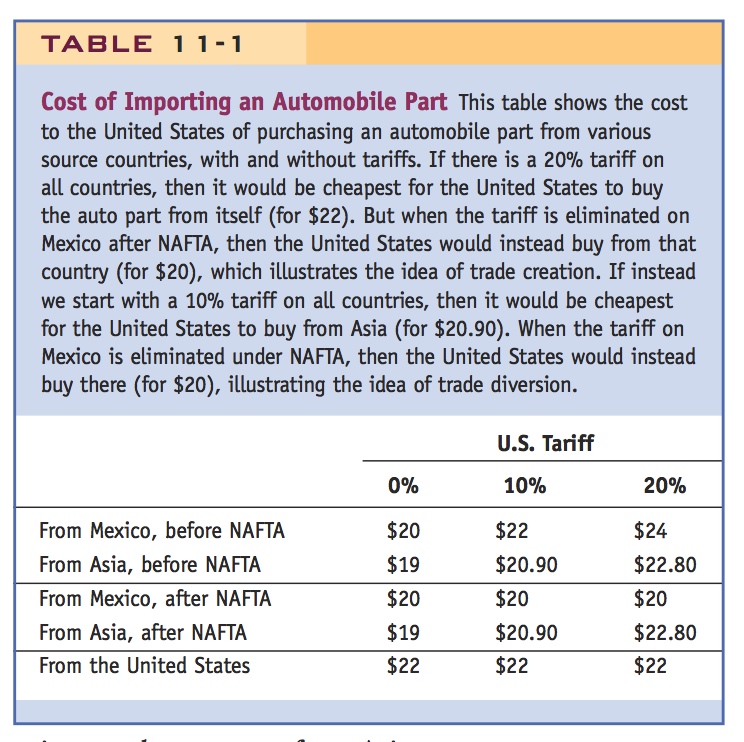
Suppose that the costs to the United States of importing an auto part from Mexico or from Asia are as shown in Table 11-1. The rightmost columns show the total costs of the part under free trade (zero tariff), with a 10% tariff and 20% tariff, respectively. Under free trade, the auto part can be produced in Mexico for $20 or in Asia for $19. Thus, Asia is the most efficient producer. If the United States purchased the part from an American supplier, it would cost $22, as shown in the last row of the table. With a tariff of 10%, the costs of importing from Mexico or Asia are increased to $22 and $20.90, respectively. Similarly, a 20% tariff would increase the cost of importing to $24 and $22.80, respectively. Under NAFTA, however, the cost of importing from Mexico is $20 regardless of the tariff.
With the data shown in Table 11-1, we can examine the effect of NAFTA on each country’s welfare. First, suppose that the tariff applied by the United States is 20%, as shown in the last column. Before NAFTA, it would have cost $24 to import the auto part from Mexico, $22.80 to import it from Asia, and $22 to produce it locally in the United States. Before NAFTA, then, producing the part in the United States for $22 is the cheapest option. With the tariff of 20%, therefore, there are no imports of this auto part into the United States.
377
Trade Creation When Mexico joins NAFTA, it pays no tariff to the United States, whereas Asia continues to have a 20% tariff applied against it. After NAFTA, the United States will import the part from Mexico for $20 because the price is less than the U.S. cost of $22. Therefore, all the auto parts will be imported from Mexico. This is an example of trade creation. The United States clearly gains from the lower cost of the auto part; Mexico gains from being able to export to the United States; and Asia neither gains nor loses, because it never sold the auto part to the United States to begin with.
Trade Diversion Now suppose instead that the U.S. tariff on auto parts is 10% (the middle column of Table 11-1). Before NAFTA, the United States can import the auto part from Mexico for $22 or from Asia for $20.90. It still costs $22 to produce the part at home. In this case, the least-cost option is for the United States to import the auto part from Asia. When Mexico joins NAFTA, however, this outcome changes. It will cost $20 to import the auto part from Mexico duty-free, $20.90 to import it from Asia subject to the 10% tariff, and $22 to produce it at home. The least-cost option is to import the auto part from Mexico. Because of the establishment of NAFTA, the United States switches the source of its imports from Asia to Mexico, an example of trade diversion.
Producer surplus in Asia falls because it loses its export sales to the United States, whereas producer surplus in Mexico rises. What about the United States? Before NAFTA, it imported from Asia at a price of $20.90, of which 10% (or $1.90 per unit) consisted of the tariff. The net-of-tariff price that Asia received for the auto parts was $19. After NAFTA the United States instead imports from Mexico, at the price of $20, but it does not collect any tariff revenue at all. So the United States gains 90¢ on each unit from paying a lower price, but it also loses $1.90 in tariff revenue from not purchasing from Asia. From this example, it seems that importing the auto part from Mexico is not a very good idea for the United States because it no longer collects tariff revenue. To determine the overall impact on U.S. welfare, we can analyze the same example in a graph.
Trade Diversion in a Graph
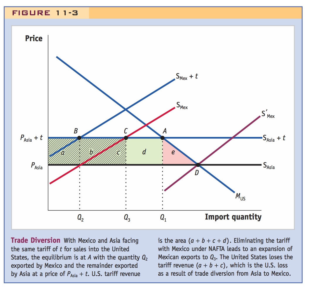
In Figure 11-3, we show the free-trade price of the auto part from Asia as PAsia, and the free-trade export supply curve from Asia as the horizontal line labeled SAsia. By treating this price as fixed, we are supposing that the United States is a small country relative to the potential supply from Asia. Inclusive of the tariff, the cost of imported parts from Asia becomes PAsia + t, and the supply curve is SAsia + t. The free-trade supply from Mexico is shown as the upward-sloping curve labeled SMex; inclusive of the tariff, the supply curve is SMex + t.
378
Before NAFTA, both Mexico and Asia face the same tariff of t. So the equilibrium imports occur at point A, where the quantity imported is Q1 and the tariff-inclusive price to the United States is PAsia + t. Of the total imports Q1, the amount Q2 comes from Mexico at point B, since under perfect competition these imports have the same tariff-inclusive price as those from Asia. Thus, tariff revenue is collected on imports from both Mexico and Asia, so the total tariff revenue is the area (a + b + c + d) in Figure 11-3.
After Mexico joins NAFTA, it is able to sell to the United States duty-free. In that case, the relevant supply curve is SMex, and imports from Mexico expand to Q3 at point C. Notice that the price charged by Mexico at point C still equals the tariff-inclusive price from Asia, which is PAsia + t, even though Mexican imports do not have any tariff. Mexico charges that price because its marginal costs have risen along its supply curve, so even though the tariff has been removed, the price of its imports to the United States has not changed.
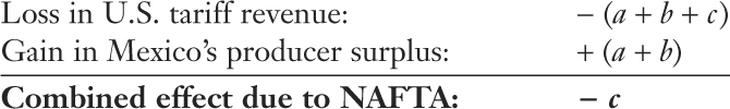
Because the imports from Mexico enter the United States duty-free, the United States loses tariff revenue of t · Q3, which is the area (a + b + c) in Figure 11-3. The price of imports to the United States has not changed, so the United States is worse off due to NAFTA by the loss in its tariff revenue. Mexico is better off because of the increase in its producer surplus from charging the price PAsia + t, without paying any tariff on its expanded amount of exports. Mexico’s producer surplus rises by (a + b), the area to the left of the supply curve SMex. If we add together the changes in U.S. and Mexican welfare, the combined change in their welfare is
379
This a very neat and counterintuitive result, so go through the argument very carefully.
So we see that the combined welfare of the United States and Mexico actually falls as a result of NAFTA. This is a very counterintuitive result because we normally expect that countries will be better off when they move toward free trade. Instead, in this example, we see that one of the countries within the regional agreement is worse off (the United States), and so much so that its fall in welfare exceeds the gains for Mexico, so that their combined welfare falls!
Interpretation of the Loss This is one of the few instances in this textbook in which a country’s movement toward free trade makes that country worse off. What is the reason for this result? Asia is the most efficient producer of auto parts in this example for units Q3 − Q2: its marginal costs equal PAsia (not including the tariff). By diverting production to Mexico, the marginal costs of Mexico’s extra exports to the United States rise from PAsia (which is the marginal cost at quantity Q2, not including the tariff) to PAsia + t (which is Mexico’s marginal cost at quantity Q3). Therefore, the United States necessarily loses from trade diversion, and by more than Mexico’s gain.
The combined loss to the United States and Mexico of area c can be interpreted as the average difference between Mexico’s marginal cost (rising from PAsia to PAsia + t) and Asia’s marginal cost (PAsia), multiplied by the extra imports from Mexico. This interpretation of the net loss area c is similar to the “production loss” or “efficiency loss” due to a tariff for a small country. However, in this case, the net loss comes from removing a tariff among the member countries of a regional agreement rather than from adding a tariff.
What you should keep in mind in this example of the adverse effects of trade diversion is that the tariff between the United States and Mexico was removed, but the tariff against imports of auto parts from Asia was maintained. So it is really only a halfway step toward free trade. We have shown that this halfway step can be bad for the countries involved rather than good. This effect of trade diversion explains why some economists oppose regional trade agreements but support multilateral agreements under the WTO.
Now provide this counterexample . . .
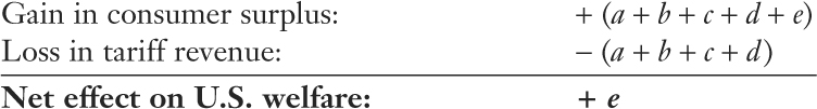
Not All Trade Diversion Creates a Loss We should stress that the loss due to a regional trade agreement in this example is not a necessary result, but a possible result, depending on our assumptions of Mexico’s marginal costs. There could also be a gain to the importing country. In Figure 11-3, for example, suppose that after joining NAFTA, Mexico has considerable investment in the auto parts industry, and its supply curve shifts to  rather than SMex. Then equilibrium imports to the United States will occur at point D, at the price PAsia, and Mexico will fully replace Asia as a supplier of auto parts. As compared with the initial situation with the tariff, the United States will lose all tariff revenue of area (a + b + c + d). But the import price drops to PAsia, so it has a gain in consumer surplus of area (a + b + c + d + e). Therefore, the net change in U.S. welfare is
380
The United States experiences a net gain in consumer surplus in this case, and Mexico’s producer surplus rises because it is exporting more.
. . . to arrive at this rule of thumb.
This case combines elements of trade diversion (Mexico has replaced Asia) and trade creation (Mexico is exporting more to the United States than total U.S. imports before NAFTA). Thus, we conclude that NAFTA and other regional trade agreements have the potential to create gains among their members, but only if the amount of trade creation exceeds the amount of trade diversion. In the following application we look at what happened to Canada and the United States when free trade opened between them, to see whether the extent of trade creation for Canada exceeded the amount of trade diversion.
Trefler’s estimates of how NAFTA affected Canada: Imports from U.S. increased by 54 percent, while imports from the rest of the world decreased by 40 percent. Since the U.S. provides 80 percent of Canada’s imports, so trade creation exceeded trade diversion by 35 percent.
Trade Creation and Diversion for Canada
In 1989, Canada formed a free-trade agreement with the United States and, five years later, entered into the North American Free Trade Agreement with the United States and Mexico. Research by Professor Daniel Trefler at the University of Toronto has analyzed the effect of these free-trade agreements on Canadian manufacturing industries. As summarized in Chapter 6, initially there was unemployment in Canada, but that was a short-term result. A decade after the free-trade agreement with the United States, employment in Canadian manufacturing had recovered and that sector also enjoyed a boom in productivity.
In his research, Trefler also estimated the amount of trade creation versus trade diversion for Canada in its trade with the United States. He found that the reduction in Canadian tariffs on U.S. goods increased imports of those goods by 54%. This increase was trade creation. However, since Canada was now buying more tariff-free goods from the United States, those tariff reductions reduced Canadian imports from the rest of the world by 40% (trade diversion). To compare these amounts, keep in mind that imports from the United States make up 80% of all Canadian imports, whereas imports from the rest of the world make up the remaining 20%. So the 54% increase in imports from the United States should be multiplied (or weighted) by its 80% share in overall Canadian imports to get the amount of trade creation. Likewise, the 40% reduction in imports from the rest of the world should be multiplied by its 20% share in Canadian imports to get trade diversion. Taking the difference between the trade created and diverted, we obtain
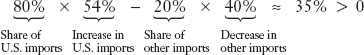
Because this calculation gives a positive number, Trefler concludes that trade creation exceeded trade diversion when Canada and the United States entered into the free-trade agreement. Therefore, Canada definitely gained from the free-trade agreement with the United States.
So NAFTA was a good thing, for Canadian manufacturing.