3 The Monetary Approach: Implications and Evidence
Applications and empirical evidence of the simple monetary model
1. Exchange Rate Forecasts Using the Simple Model
The monetary model suggests that forecasts of money and real growth could be used to forecast exchange rates. Two warnings: (1) it is hard to forecast these things; (2) this is a long-run model, where PPP is assumed to hold, so it may not work well in the short run.
a. Forecasting Exchange Rates: An Example
Suppose monetary and real growth are zero, so the exchange rate is initially constant. What happens if there is . . . ?
Case 1. A one-time unanticipated increase in M of 10 percent. Since Y is constant, P increases by 10 percent. By PPP, E increases by 10 percent.
Case 2. An unanticipated increase in the growth rate of M. Since Y is constant, Prices increase at the same rate as the money supply. By PPP, the exchange rate increases at the same rate too. Money growth causes inflation, which in turn depreciates the currency.
The monetary approach is the workhorse model in the study of long-run exchange rate movements. In this section, we look at some applications and empirical evidence.
Exchange Rate Forecasts Using the Simple Model
An important application of the monetary approach to exchange rate determination is to provide a forecast of the future exchange rate. Remember from the previous chapter that foreign exchange (forex) market arbitragers need such a forecast to be able to make arbitrage calculations using uncovered interest parity. Using Equation (3-3), we can see that a forecast of future exchange rates (the left-hand side) can be constructed as long as we know how to forecast future money supplies and real income (the right-hand side).
83
In practice, this is why expectations about money and real income in the future attract so much attention in the financial media, and especially in the forex market. The discussion returns with obsessive regularity to two questions. The first question—What are central banks going to do?—leads to all manner of attempts to decode the statements of central bank officials. The second question—How is the economy expected to grow in real terms?—leads to a keen interest in any economic indicators, such as productivity or investment, that might hint at changes in the rate of income growth.
Digress to talk about how economists use models to make predictions about how changes in exogenous things affect endogenous things. But making forecasts in the real world is tricky because (1) you need to know the correct model for the given problem, and (2) you need to know what the exogenous things are likely to do.
Any such forecasts come with at least two major caveats. First, there is great uncertainty in trying to answer these questions, and forecasts of economic variables years in the future are inevitably subject to large errors. Nonetheless, this is one of the key tasks of financial markets. Second, whenever one uses the monetary model for forecasting, one is answering a hypothetical question: What path would exchange rates follow from now on if prices were flexible and PPP held? As forecasters know, in the short run there might be deviations from this prediction about exchange rate changes, but in the longer run, we expect the prediction will supply a more reasonable guide.
Also ask them to think through the effects of changes in the level and growth rate of income.
Forecasting Exchange Rates: An Example To see how forecasting might work, let’s look at a simple scenario and focus on what would happen under flexible prices. Assume that U.S. and European real income growth rates are identical and equal to zero (0%) so that real income levels are constant. Assume also that the European money supply is constant. If the money supply and real income in Europe are constant, then the European price level is constant, and European inflation is zero, as we can see from Equation (3-5). These assumptions allow us to perform a controlled thought-experiment, and focus on changes on the U.S. side of the model, all else equal. Let’s look at two cases.
Case 1: A one-time unanticipated increase in the money supply. In the first, and simpler, case, suppose at some time T that the U.S. money supply rises by a fixed proportion, say, 10%, all else equal. Assuming that prices are flexible, what does our model predict will happen to the level of the exchange rate after time T? To spell out the argument in detail, we look at the implications of our model for some key variables.
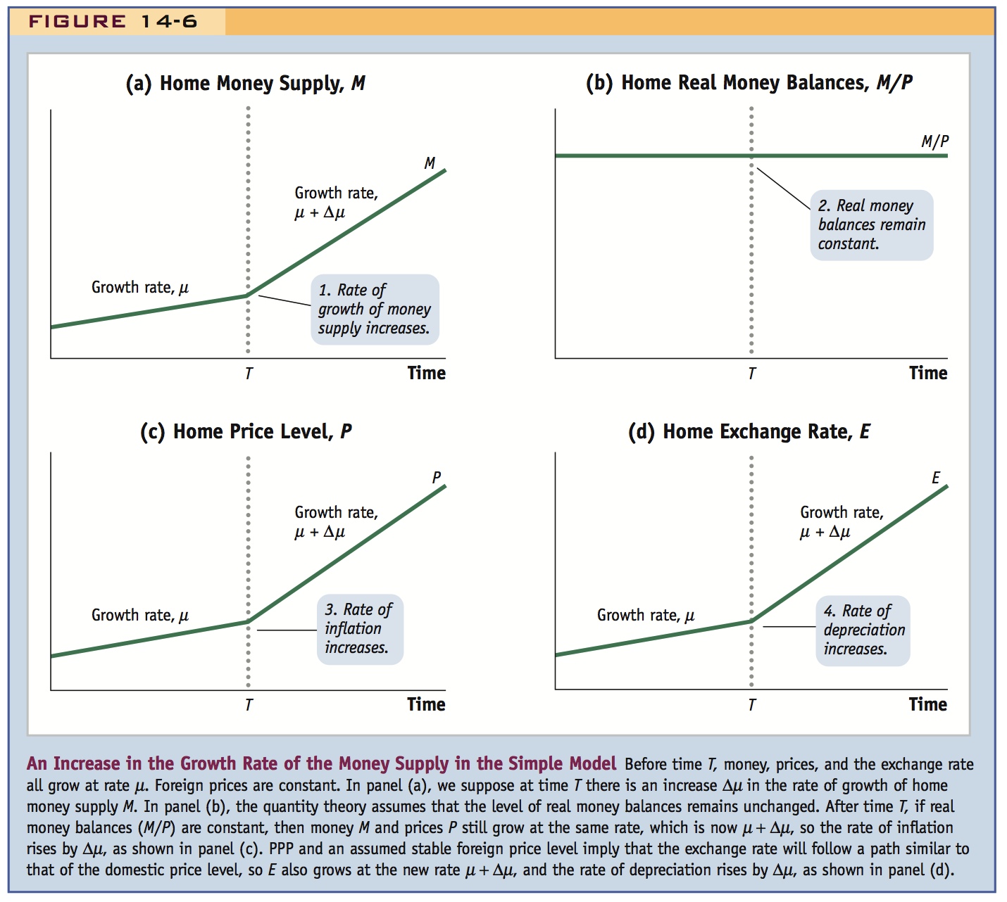
We've actually done these already when we thought about Equation 14-3. But going through these pictures will reinforce the results, and the steps enumerated here make the causal mechanism crystal clear.
Notice that because money demand is interest inelastic the price level does not jump at time zero.
- There is a 10% increase in the money supply M.
- Real money balances M/P remain constant, because real income is constant.
- These last two statements imply that price level P and money supply M must move in the same proportion, so there is a 10% increase in the price level P.
- PPP implies that the exchange rate E and price level P must move in the same proportion, so there is a 10% increase in the exchange rate E; that is, the dollar depreciates by 10%.
A quicker solution uses the fundamental equation of the monetary approach at Equation (3-3): the price level and exchange rate are proportional to the money supply, all else equal.
Case 2: An unanticipated increase in the rate of money growth. The model also applies to more complex scenarios. Consider a second case in which the U.S. money supply is not constant, but grows at a steady fixed rate μ. Then suppose we learn at time T that the United States will raise the rate of money supply growth from some previously fixed rate μ to a slightly higher rate μ + Δμ. How would people expect the exchange rate to behave, assuming price flexibility? Let’s work through this case step by step:
84
- Money supply M is growing at a constant rate.
- Real money balances M/P remain constant, as before.
- These last two statements imply that price level P and money supply M must move in the same proportion, so P is always a constant multiple of M.
- PPP implies that the exchange rate E and price level P must move in the same proportion, so E is always a constant multiple of P (and hence of M).
Corresponding to these four steps, the four panels of Figure 14-6 illustrate the path of the key variables in this example. This figure shows that if we can forecast the money supply at any future period as in (a), and if we know real money balances remain constant as in (b), then we can forecast prices as in (c) and exchange rates as in (d). These forecasts are good in any future period, under the assumptions of the monetary approach. Again, Equation (3-3) supplies the answer more quickly; under the assumptions we have made, money, prices, and exchange rates all move in proportion to one another.
85
Cross-sectional evidence supporting the hypothesis that money growth should be of the same size as inflation and depreciation over long periods.
Conclusion: Money growth = inflation = depreciation over long periods . . .
Evidence for the Monetary Approach
The monetary approach to prices and exchange rates suggests that, all else equal, increases in the rate of money supply growth should be the same size as increases in the rate of inflation and the rate of exchange rate depreciation. Looking for evidence of this relationship in real-world data is one way to put this theory to the test.
The scatterplots in Figure 14-7 and Figure 14-8 show data from 1975 to 2005 for a large sample of countries. The results offer fairly strong support for the monetary theory. All else equal, Equation (3-6) predicts that an x% difference in money growth rates (relative to the United States) should be associated with an x% difference in inflation rates (relative to the United States) and an x% depreciation of the home exchange rate (against the U.S. dollar). If this association were literally true in the data, then each country in the scatterplot would be on the 45-degree line. This is not exactly true, but the actual relationship is very close and offers some support for the monetary approach.


One reason the data do not sit on the 45-degree line is that all else is not equal in this sample of countries. In Equation (3-6), countries differ not only in their relative money supply growth rates but also in their real income growth rates. Another explanation is that we have been assuming that the money demand parameter L is constant, and this may not be true in reality. This is an issue we must now confront.9
86
PPP works very well in hyperinflations, even in the short run. The simple model assumes money demand is stable. However, it falls during hyperinflations, as people try to economize on their money holdings. Even in the short run, it is implausible to assume that money demand is always stable.
Hyperinflations
The monetary approach assumes long-run PPP, which has some support, as we saw in Figure 14-2. But we have been careful to note, again, that PPP generally works poorly in the short run. However, there is one notable exception to this general failure of PPP in the short run: hyperinflations.
Economists traditionally define a hyperinflation as occurring when the inflation rate rises to a sustained rate of more than 50% per month (which means that prices are doubling every 51 days). In common usage, some lower-inflation episodes are also called hyperinflations; for example, an inflation rate of 1,000% per year is a common rule of thumb (when inflation is “only” 22% per month).
There have been many hyperinflations worldwide since the early twentieth century. They usually occur when governments face a budget crisis, are unable to borrow to finance a deficit, and instead choose to print money to cover their financing needs. The situation is not sustainable and usually leads to economic, social, or political crisis, which is eventually resolved with a return to price stability. (For more discussion of hyperinflations and their consequences, see Side Bar: Currency Reform and Headlines: The First Hyperinflation of the Twenty-First Century.)
Celia Dugger’s article from NYT on hyperinflation in Zimbabwe.
87
Describes currency reforms in response to hyperinflations
Currency Reform
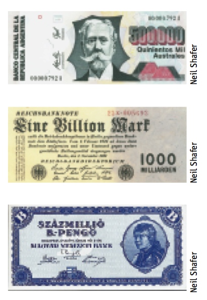
Hyperinflations help us understand how some currencies become extinct if they cease to function well and lose value rapidly. Dollarization in Ecuador is a recent example. Other currencies survive such traumas, only to be reborn. But the low denomination bills—the ones, fives, tens—usually become essentially worthless and normal transactions can require you to be a millionaire. The elimination of a few pesky zeros might then be a good idea. A government may then redenominate a new unit of currency equal to 10N (10 raised to the power N) old units.
Sometimes N can get quite large. In the 1980s, Argentina suffered hyperinflation. On June 1, 1983, the peso argentino replaced the (old) peso at a rate of 10,000 to 1. Then on June 14, 1985, the austral replaced the peso argentino at 1,000 to 1. Finally, on January 1, 1992, the convertible peso replaced the austral at a rate of 10,000 to 1 (i.e., 10,000,000,000 old pesos). After all this, if you had owned 1 new peso in 1983 (and had changed it into the later monies), it would have lost 99.99997% of its U.S. dollar value by 2003.
In 1946 the Hungarian pengö became so worthless that the authorities no longer printed the denomination on each note in numbers, but only in words—perhaps to avert distrust (unsuccessful), to hide embarrassment (also unsuccessful), or simply because there wasn’t room to print all those zeros. By July 15, 1946, there were 76,041,000,000,000,000,000,000,000 pengö in circulation. A stable new currency, the forint, was finally introduced on July 26, 1946, with each forint worth 400,000 quadrillion pengö (4 × 1020 = 400,000,000,000,000,000,000 pengö). The dilution of the Zimbabwean dollar from 2005 to 2009 was even more extreme, as the authorities lopped off 25 zeros in a series of reforms before the currency finally vanished from use.
... and in hyperinflations, where monetary forces might be expected to dominate
PPP in Hyperinflations Each of these crises provides a unique laboratory for testing the predictions of the PPP theory. The scatterplot in Figure 14-9 looks at the data using changes in levels (from start to finish, expressed as multiples). The change in the exchange rate (with the United States) is on the vertical axis and the change in the price level (compared with the United States) is on the horizontal axis. Because of the huge changes involved, both axes use log scales in powers of 10. For example, 1012 on the vertical axis means the exchange rate rose (the currency depreciated) by a factor of a trillion against the U.S. dollar during the hyperinflation.

If PPP holds, changes in prices and exchange rates should be equal and all observations would be on the 45-degree line. The changes follow this pattern very closely, providing support for PPP. What the hyperinflations have in common is that a very large depreciation was about equal to a very large inflation differential. In an economy with fairly stable prices and exchange rates, large changes in exchange rates and prices only develop over the very long run of years and decades; in a hyperinflation, large inflations and large depreciations are compressed into the short run of years or months, so this is one case where PPP holds quite well even in the short run.
Some price changes were outrageously large. Austria’s hyperinflation of 1921 to 1922 was the first one on record, and prices rose by a factor of about 100 (102). In Germany from 1922 to 1923, prices rose by a factor of about 20 billion (2 × 10¹⁰); in the worst month, prices were doubling on average every two days. In Hungary from 1945 to 1946, pengö prices rose by a factor of about 4 septillion (4 × 1027), the current record, and in July 1946, prices were doubling on average every 15 hours. Serbia’s inflation from 1992 to 1994 came close to breaking the record for cumulative price changes, as did the most recent case in Zimbabwe. In comparison, Argentina’s 700-fold inflation and Brazil’s 200-fold inflation from 1989 to 1990 look modest.
88
Money Demand in Hyperinflations There is one other important lesson to be learned from hyperinflations. In our simple monetary model, the money demand parameter L was assumed to be constant and equal to  . This implied that real money balances were proportional to real income, with
  as shown in Equation (3-5). Is this assumption of stable real money balances justified?
This is the perfect way to motivate an interest elastic money demand.
The evidence shown in Figure 14-10 suggests this assumption is not justified, based on a subset of the hyperinflations. For each point, on the horizontal axis of this figure, we see the peak monthly inflation rate (the moment when prices were rising most rapidly); on the vertical axis, we see the level of real money balances in that month relative to their initial level (in the month just before the hyperinflation began). If real money balances were stable, there should be no variation in the vertical dimension aside from fluctuations in real income. But there is, and with a clear pattern: the higher the level of inflation, the lower the level of real money balances. These declines are far too severe to be explained by just the fall in real incomes experienced during hyperinflations, though such income declines did occur.

This finding may not strike you as very surprising. If prices are doubling every few days (or every few hours), the money in people’s pockets is rapidly turning into worthless pieces of paper. They will try to minimize their money holdings—and will do so even more as inflation rises higher and higher, just as the figure shows. It becomes just too costly to hold very much money, despite one’s need to use it for transactions.
89
If you thought along these lines, you have an accurate sense of how people behave during hyperinflations. You also anticipated the extensions to the simple model that we make in the next section so it is more realistic. Even during “normal” inflations—situations that are less pathological than a hyperinflation—it is implausible to assume that real money balances are perfectly stable. In our extension of the simple model, we will assume that people make the trade-off highlighted previously: comparing the benefits of holding money for transactions purposes with the costs of holding money as compared with other assets.