4 Money, Interest Rates, and Prices in the Long Run: A General Model
Now drop the assumption that money demand is stable, and allow it to vary with the interest rate.
1. The Demand for Money: The General Model
Motivate the nominal interest rate i as the opportunity cost of holding money. Then Md⁄P = L(i)Y, where L(i) is decreasing in i.
2. Long-Run Equilibrium in the Money Market
M⁄P = L(i)Y, but what determines i in the long run?
3. Inflation and Interest Rates in the Long Run
Taking expectations, PPP says 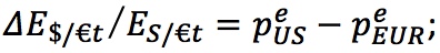 UIP says
 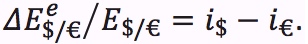 Put them together to find
 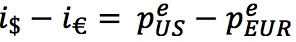 Thus the Fisher effect: An increase in expected inflation will raise interest rates by the same amount. This explains why money demand falls in hyperinflations: Inflation raises interest rates, which reduces money demand.
4. Real Interest Parity
Rewrite the previous result as 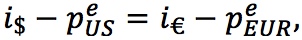 or
or 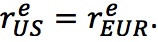 . Convergence of real goods prices, via PPP, should also make real interest rates converge. Call the common long-run real rate Then the Fisher effect implies that each country’s long-run nominal rate should equal the expected world real rate plus its expected inflation, e.g.,
 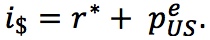 .
.
So far we have a long-run theory that links exchange rates to the price levels in each country: PPP. We also have a simple long-run monetary model that links price levels in each country to money supply and demand: the quantity theory.
These building blocks provide some basic intuition for the links between price levels, money, and exchange rates. The trouble is that the quantity theory’s assumption—that the demand for money is stable—is implausible. In this section, we explore a more general model that addresses this shortcoming by allowing money demand to vary with the nominal interest rate. But this theory, in turn, brings another variable into play: How is the nominal interest rate determined in the long run? Answering this question will lead us to consider the links between inflation and the nominal interest rate in an open economy. With these new models in hand, we then return to the question of how best to understand what determines exchange rates in the long run.
90
The First Hyperinflation of the Twenty-First Century
By 2007 Zimbabwe was almost at an economic standstill, except for the printing presses churning out banknotes. A creeping inflation—58% in 1999, 132% in 2001, 385% in 2003, and 586% in 2005—was about to become hyperinflation, and the long-suffering people faced an accelerating descent into even greater chaos. Three years later, shortly after this news report, the local currency disappeared from use, replaced by U.S. dollars and South African rand.
…Zimbabwe is in the grip of one of the great hyperinflations in world history. The people of this once proud capital have been plunged into a Darwinian struggle to get by. Many have been reduced to peddlers and paupers, hawkers and black-market hustlers, eating just a meal or two a day, their hollowed cheeks a testament to their hunger.
Like countless Zimbabweans, Mrs. Moyo has calculated the price of goods by the number of days she had to spend in line at the bank to withdraw cash to buy them: a day for a bar of soap; another for a bag of salt; and four for a sack of cornmeal.
The withdrawal limit rose on Monday, but with inflation surpassing what independent economists say is an almost unimaginable 40 million percent, she said the value of the new amount would quickly be a pittance, too.
“It’s survival of the fittest,” said Mrs. Moyo, 29, a hair braider who sells the greens she grows in her yard for a dime a bunch. “If you’re not fit, you will starve.”
Economists here and abroad say Zimbabwe’s economic collapse is gaining velocity, radiating instability into the heart of southern Africa. As the bankrupt government prints ever more money, inflation has gone wild, rising from 1,000 percent in 2006 to 12,000 percent in 2007…. In fact, Zimbabwe’s hyperinflation is probably among the five worst of all time, said Jeffrey D. Sachs, a Columbia University economics professor, along with Germany in the 1920s, Greece and Hungary in the 1940s and Yugoslavia in 1993….
Basic public services, already devastated by an exodus of professionals in recent years, are breaking down on an ever larger scale as tens of thousands of teachers, nurses, garbage collectors and janitors have simply stopped reporting to their jobs because their salaries, more worthless literally by the hour, no longer cover the cost of taking the bus to work….
The bodies of paupers in advanced states of decay were stacking up in the mortuary at Beitbridge District Hospital because not even government authorities were seeing to their burial…. Harare Central Hospital slashed admissions by almost half because so much of its cleaning staff could no longer afford to get to work.
Most of the capital, though lovely beneath its springtime canopy of lavender jacaranda blooms, was without water because the authorities had stopped paying the bills to transport the treatment chemicals. Garbage is piling up uncollected. Sixteen people have died in an outbreak of cholera in nearby Chitungwiza, spread by contaminated water and sewage….
Vigilantes in Kwekwe killed a man suspected of stealing two chickens, eggs and a bucket of corn…. And traditional chiefs complained about corrupt politicians and army officers who sold grain needed for the hungry to the politically connected instead.
Source: Celia Dugger, "Life in Zimbabwe: Wait for Useless Money, Then Scour for Food." From The New York Times, October 2, 2008 © 2008 The New York Times. All rights reserved. Used by permission and protected by the Copyright Laws of the United States. The printing, copying, redistribution, or retransmission of this Content without express written permission is prohibited.
The Demand for Money: The General Model
The general model of money demand is motivated by two insights, the first of which carries over from the quantity theory, the simple model we studied earlier in this chapter.
91
Emphasize that this is the nominal interest rate.
- There is a benefit from holding money. As is true in the simple quantity theory, the benefit of money is that individuals can conduct transactions with it, and we continue to assume that transactions demand is in proportion to income, all else equal.
- There is a cost to holding money. The nominal interest rate on money is zero, imoney = 0. By holding money and not earning interest, people incur the opportunity cost of holding money. For example, an individual could hold an interest-earning asset paying i$. The difference in nominal returns between this asset and money would be i$ − imoney = i$ > 0. This is one way of expressing the opportunity cost.
Moving from the individual or household level up to the macroeconomic level, we can infer that aggregate money demand in the economy as a whole will behave similarly:
Draw the graphs on the next page.
All else equal, a rise in national dollar income (nominal income) will cause a proportional increase in transactions and, hence, in aggregate money demand.
All else equal, a rise in the nominal interest rate will cause the aggregate demand for money to fall.
Again, a possible historical digression: Keynes was a student of Marshall's, who first suggested that money demand should depend upon interest rates. This is just a Cambridge money demand where L is allowed to be a function of of i.
Thus, we arrive at a general model in which money demand is proportional to nominal income, and is a decreasing function of the nominal interest rate:
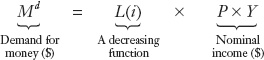
Recall that, formerly, in the quantity theory, the parameter L (the liquidity ratio, the amount of money needed for transactions per dollar of nominal GDP) was a constant. In this general model, we assume that L is a decreasing function of the nominal interest rate i. Dividing by P, we can derive the demand for real money balances:
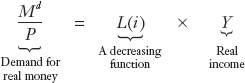
Figure 14-11(a) shows a typical real money demand function of this form, with the quantity of real money balances demanded on the horizontal axis and the nominal interest rate on the vertical axis. The downward slope of the demand curve reflects the inverse relationship between the demand for real money balances and the nominal interest rate at a given level of real income (Y).

Figure 14-11(b) shows what happens when real income increases from Y1 to Y2. When real income increases (by x%), the demand for real money balances increases (by x%) at each level of the nominal interest rate and the curve shifts.
Long-Run Equilibrium in the Money Market
The money market is in equilibrium when the real money supply (determined by the central bank) equals the demand for real money balances (determined by the nominal interest rate and real income):

92
We will continue to assume that prices are flexible in the long run and that they adjust to ensure that equilibrium is maintained.
What determines i in the long run? Irving Fisher.
We now have a model that describes equilibrium in the money market which will help us on the way to understanding the determination of the exchange rate. Before we arrive at the long-run exchange rate, however, we need one last piece to the puzzle. Under the quantity theory, the nominal interest rate was ignored. Now, in our general model, it is a key variable in the determination of money demand. So we need a theory to tell us what the level of the nominal interest rate i will be in the long run. Once we have solved this problem, we will be able to apply this new, more complex, but more realistic model of the money market to the analysis of exchange rate determination in the long run.
Inflation and Interest Rates in the Long Run
The tools we need to determine the nominal interest rate in an open economy are already at hand. So far in this chapter, we have developed the idea of purchasing power parity (PPP), which links prices and exchange rates. In the last chapter, we developed another parity idea, uncovered interest parity (UIP), which links exchange rates and interest rates. With only these two relationships in hand, PPP and UIP, we can derive a powerful and striking result concerning interest rates that has profound implications for our study of open economy macroeconomics.
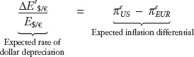
Relative PPP, as indicated in Equation (3-2), states that the rate of depreciation equals the inflation differential at time t. When market actors use this equation to forecast future exchange rates, we use a superscript e to denote such expectations. Equation (3-2) is recast to show expected depreciation and inflation at time t:
93
Since we are interested in forecasts, combine ex ante relative PPP with UIP to derive the Fisher equation. They may have seen the Fisher equation for a closed economy, but it is nice to derive it directly from PPP and UIP.
Next we recall that UIP in the approximate form (Equation 2-3) can be rearranged to show that the expected rate of depreciation equals the interest differential at time t:
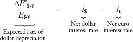
This way of writing the UIP equation says that traders will be indifferent to a higher U.S. interest rate relative to the euro interest rates (making U.S. deposits look more attractive) only if the higher U.S. rate is offset by an expected dollar depreciation (making U.S. deposits look less attractive). For example, if the U.S. interest rate is 4% and the euro interest rate is 2%, the interest differential is 2% and the forex market can be in equilibrium only if traders expect a 2% depreciation of the U.S. dollar against the euro, which would exactly offset the higher U.S. interest rate.
The Fisher Effect
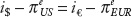
Because the left sides of the previous two equations are equal, the right sides must also be equal. Thus, the nominal interest differential equals the expected inflation differential:

What does this important result say? To take an example, suppose expected inflation is 4% in the United States and 2% in Europe. The inflation differential on the right is then +2% (4% − 2% = +2%). If interest rates in Europe are 3%, then to make the interest differential the same as the inflation differential, +2%, the interest rate in the United States must equal 5% (5% − 3% = +2%).
Now suppose expected inflation in the United States changes, rising by one percentage point to 5%. If nothing changes in Europe, then the U.S. interest rate must also rise by one percentage point to 6% for the equation to hold. In general, this equation predicts that changes in the expected rate of inflation will be fully incorporated (one for one) into changes in nominal interest rates.
All else equal, a rise in the expected inflation rate in a country will lead to an equal rise in its nominal interest rate.
This result is known as the Fisher effect, named for the American economist Irving Fisher (1867–1947). Note that because this result depends on an assumption of PPP, it is therefore likely to hold only in the long run.
94
Say that now we have a link between inflation (and hence depreciation) and money demand, as suggested by the hyperinflations.
The Fisher effect makes clear the link between inflation and interest rates under flexible prices, a finding that is widely applicable. For a start, it makes sense of the evidence we just saw on money holdings during hyperinflations (see Figure 14-10). As inflation rises, the Fisher effect tells us that the nominal interest rate i must rise by the same amount; the general model of money demand then tells us that L(i) must fall because it is a decreasing function of i. Thus, for a given level of real income, real money balances must fall as inflation rises.
In other words, the Fisher effect predicts that the change in the opportunity cost of money is equal not just to the change in the nominal interest rate but also to the change in the inflation rate. In times of very high inflation, people should, therefore, want to reduce their money holdings—and they do.
Real Interest Parity
As just described, the Fisher effect tells us something about nominal interest rates, but we can quickly derive the implications for real interest rates, too. Rearranging the last equation, we find
The expressions on either side of this equation might look familiar from previous courses in macroeconomics. When the inflation rate (π) is subtracted from a nominal interest rate (i), the result is a real interest rate (r), the inflation-adjusted return on an interest-bearing asset. Given this definition, we can simplify the last equation further. On the left is the expected real interest rate in the United States 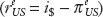 . On the right is the expected real interest rate in Europe
  .
.
Thus, using only two assumptions, PPP and UIP, we have shown that

This remarkable result states the following: if PPP and UIP hold, then expected real interest rates are equalized across countries.
This powerful condition is called real interest parity and because it depends on an assumption of PPP, it is therefore likely to hold only in the long run.10
We have arrived at a strong conclusion about the potential for globalization to cause convergence in economic outcomes, because real interest parity implies the following: arbitrage in goods and financial markets alone is sufficient, in the long run, to cause the equalization of real interest rates across countries.
This is an interesting point that should be highlighted.
We have considered two locations, but this argument applies to all countries integrated into the global capital market. In the long run, they will all share a common expected real interest rate, the long-run expected world real interest rate denoted r*, so
95
From now on, unless indicated otherwise, we treat r* as a given, exogenous variable, something outside the control of a policy maker in any particular country.11
Under these conditions, the Fisher effect is even clearer, because, by definition,

Thus, in each country, the long-run expected nominal interest rate is the long-run world real interest rate plus that country’s expected long-run inflation rate. For example, if the world real interest rate is r* = 2%, and the country’s long-run expected inflation rate goes up by two percentage points from 3% to 5%, then its long-run nominal interest rate also goes up by two percentage points from the old level of 2 + 3 = 5% to a new level of 2 + 5 = 7%.
Cross-sectional evidence supporting the Fisher effect and real interest parity in the long run.
5. The Fundamental Equation Under the General Model
Allowing for interest elastic money demand: 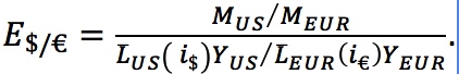 .
.
6. Exchange Rate Forecasts Using the General Model
Consider an increase in the money growth rate starting at a time T. Since Y is constant, inflation increases. By the Fisher effect, this raises nominal interest rates. This lowers money demand, so the price level jumps up discontinuously at T; after that it increases at the same growth rate as money. PPP then implies that the exchange rate will mimic the dynamics of the price level.
a. Looking Ahead
Suppose that people expect there will be an increase in the money growth rate. This fuels expectations of inflation. If people expected PPP to hold in the long run, they will deduce that the currency will depreciate in the future. UIP then implies that people will sell dollars to acquire foreign assets. This would cause the dollar to depreciate today even though the money supply hasn’t changed yet.
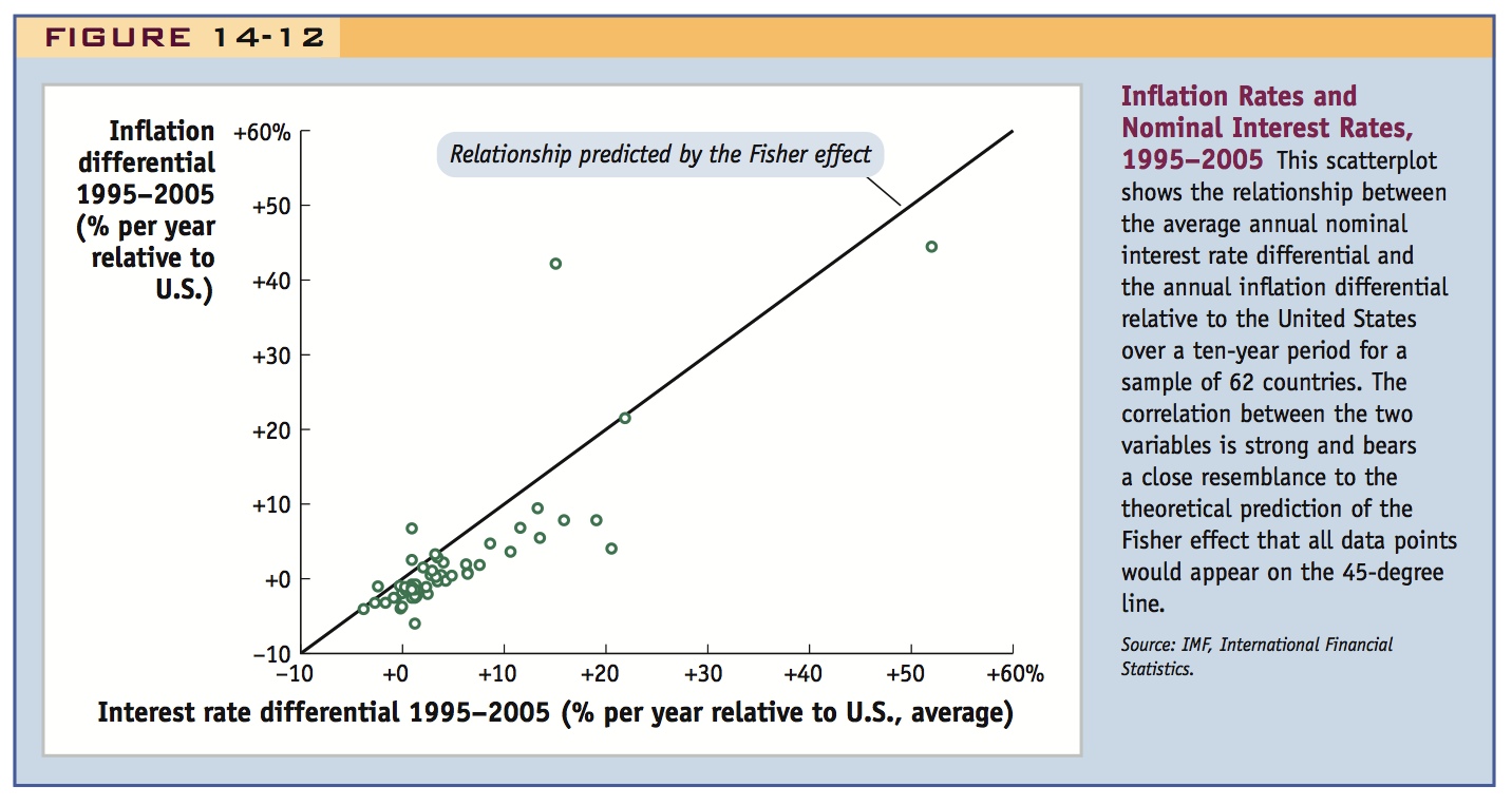
Evidence on the Fisher Effect
Are the Fisher effect and real interest parity supported by empirical evidence? One might expect a problem here. We derived them from purchasing power parity. The evidence we have seen on PPP offers support only in the long run. Thus, we do not expect the Fisher effect and real interest parity to hold exactly in the short run, but we might expect them to hold (at least approximately) in the long run.
Figure 14-12 shows that the Fisher effect is close to reality in the long run: on average, countries with higher inflation rates tend to have higher nominal interest rates, and the data line up fairly well with the predictions of the theory. Figure 14-13 shows that, for three developed countries, real interest parity holds fairly well in the long run: real interest differentials are not always zero, but they tend to fluctuate around zero in the long run. This could be seen as evidence in favor of long-run real interest parity.

96
The Fundamental Equation Under the General Model
Say that since the Fisher effect follows from PPP it should only be expected to hold in the long run, but it seems to.
Now that we understand how the nominal interest rate is determined in the long run, our general model is complete. This model differs from the simple model (the quantity theory) only by allowing L to vary as a function of the nominal interest rate i.
Here too it would help to put Figures 14-1 and 14-5 together, together with interest rates affecting money demands in the two countries. This will help clarify the causal linkages. Then use i = r* + pi and relative PPP to suggest that expected future depreciation might affect the current spot rate--adding yet another "arrow" to the flow chart.
We can therefore update our fundamental equations to allow for this change in how we treat L. For example, the fundamental equation of the monetary approach to exchange rates, Equation (3-3), can now be suitably modified:
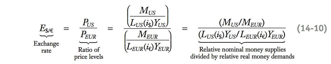
Students like this because it reveals that what is happening now depends upon what people expect to happen in the future.
What have we gained from this refinement? We know that the simple model will remain valid for cases in which nominal interest rates remain unchanged in the long run. It is only when nominal interest rates change that the general model has different implications, and we now have the right tools for that situation. To put those tools to work, we revisit the example of an exchange rate forecasting problem we encountered earlier in this chapter.
97
Exchange Rate Forecasts Using the General Model
Earlier in the chapter, we looked at two forecasting problems under the assumption of flexible prices. The first was a one-time unanticipated change in an otherwise constant U.S. money supply. Under the assumptions we made (stable real income in both countries and stable European money supply), this change caused a one-time increase in the U.S. price level but did not lead to a change in U.S. inflation (which was zero before and after the event).
The Fisher effect tells us that if inflation rates are unchanged, then, in the long run, nominal interest rates remain unchanged. Thus, the predictions of the simple model remain valid. But in the second and more complex forecasting problem, there was a one-time unanticipated change in the U.S. money growth rate that did lead to a change in inflation. It is here that the general model makes different predictions.
Earlier we assumed that U.S. and European real income growth rates are identical and equal to zero (0%), so real income levels are constant. We also assumed that the European money supply is constant, so that the European price level is constant, too. This allowed us to focus on changes on the U.S. side of the model, all else equal.
We now reexamine the forecasting problem for the case in which there is an increase in the U.S. rate of money growth. We learn at time T that the United States is raising the rate of money supply growth from some fixed rate μ to a slightly higher rate μ + Δμ.
This is a neat example, but it is complicated so take your time explaining it: you have to use all the pieces of the puzzle. Also, emphasize the jump in the price level at time zero.
For example, imagine an increase from 2% to 3% growth, so Δμ = 1%. How will the exchange rate behave in the long run? To solve the model, we make a provisional assumption that U.S. inflation rates and interest rates are constant before and after time T and focus on the differences between the two periods caused by the change in money supply growth. The story is told in Figure 14-14:

- The money supply is growing at a constant rate. If the interest rate is constant in each period, then real money balances M/P remain constant, by assumption, because L(i)Y is then a constant. If real money balances are constant, then M and P grow at the same rate. Before T that rate is μ = 2%; after T that rate is μ + Δμ = 3%. That is, the U.S. inflation rate rises by an amount Δμ = 1% at time T.
- As a result of the Fisher effect, U.S. interest rates also rise by Δμ = 1% at time T. Consequently, real money balances M/P must fall at time T because L(i)Y will decrease as i increases.
- In (a) we have described the path of M. In (b) we found that M/P is constant up to T, then drops suddenly, and then is constant after time T. What path must the price level P follow? Up to time T, it is a constant multiple of M; the same applies after time T, but the constant has increased. Why? The nominal money supply grows smoothly, without a jump. So if real money balances drop down discontinuously at time T, the price level must jump up discontinuously at time T. The intuition for this is that the rise in inflation and interest rates at time T prompts people to instantaneously demand less real money, but because the supply of nominal money is unchanged, the price level has to jump up. Apart from this jump, P grows at a constant rate; before T that rate is μ = 2%; after T that rate is μ + Δμ = 3%.
- PPP implies that E and P must move in the same proportion, so E is always a constant multiple of P. Thus, E jumps like P at time T. Apart from this jump, E grows at a constant rate; before T that rate is μ = 2%; after T that rate is μ + Δμ = 3%.
98
Corresponding to these four steps, Figure 14-14 illustrates the path of the key variables in this example. (Our provisional assumption of constant inflation rates and interest rates in each period is satisfied, so the proposed solution is internally consistent.)
Comparing Figure 14-14 with Figure 14-6, we can observe the subtle qualitative differences between the predictions of the simple quantity theory and those of the more general model. Shifts in the interest rate introduce jumps in real money demand. Because money supplies evolve smoothly, these jumps end up being reflected in the price levels and hence—via PPP—in exchange rates. The Fisher effect tells us that these interest rate effects are ultimately the result of changes in expected inflation.
99
Try adding all this to the expanded flowchart described in the comments above, to emphasize the importance of expectations.
If you want to be adventurous, ask them to think through the effects of an expected FUTURE increase in the money growth rate.
Looking Ahead We can learn a little more by thinking through the market mechanism that produces this result. People learn at time T that money growth will be more rapid in the United States. This creates expectations of higher inflation in the United States. If people believe PPP holds in the long run, they will believe higher future inflation will cause the U.S. currency to depreciate in the future. This prospect makes holding dollars less attractive, by UIP. People try to sell dollars, and invest in euros. This creates immediate downward pressure on the dollar—even though at time T itself the supply of dollars does not change at all! This lesson underlines yet again the importance of expectations in determining the exchange rate. Even if actual economic conditions today are completely unchanged, news about the future affects today’s exchange rate. This crucial insight can help us explain many phenomena relating to the volatility and instability in spot exchange rates, an idea we develop further in the chapters that follow.