3 The Asset Approach: Applications and Evidence
1. The Asset Approach to Exchange Rates: Graphical Solution
a. The U.S. Money Market
The usual money demand/supply picture, with an exogenous price level
b. The Market for Foreign Exchange
The graphical depiction of the FX market (with DR and FR curves) developed in Section 1.
c. Capital Mobility is Crucial
Capital controls would preclude arbitrage, so UIP would not hold.
d. Putting the Model to Work
Equilibrium in the money market determines the domestic interest rate. Given the FR curve in the FX market (i.e., given the foreign interest rate and the expected future spot rate), this determines the spot rate.
2. Short-Run Policy Analysis
a. A Temporary Shock to the Home Money Supply
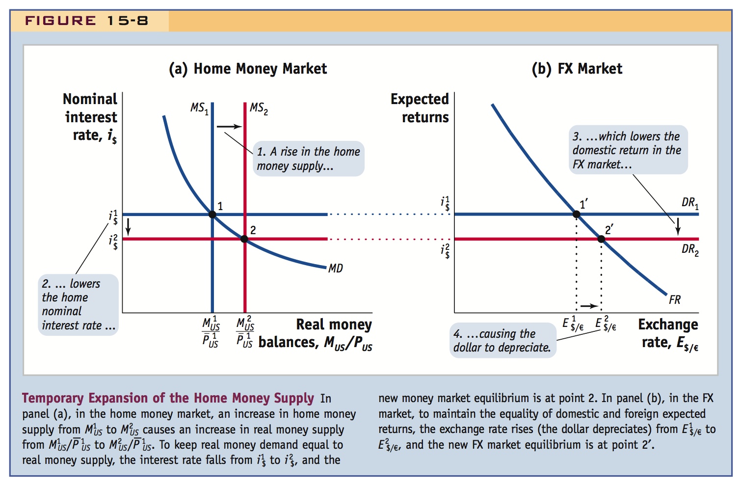
If there is a temporary increase in MU.S., the U.S. interest rate falls. DR shifts down: Capital flows to Europe, so the dollar depreciates. Notice that the expected future spot rate does not change, since the shock is temporary.
b. A Temporary Shock to the Foreign Money Supply
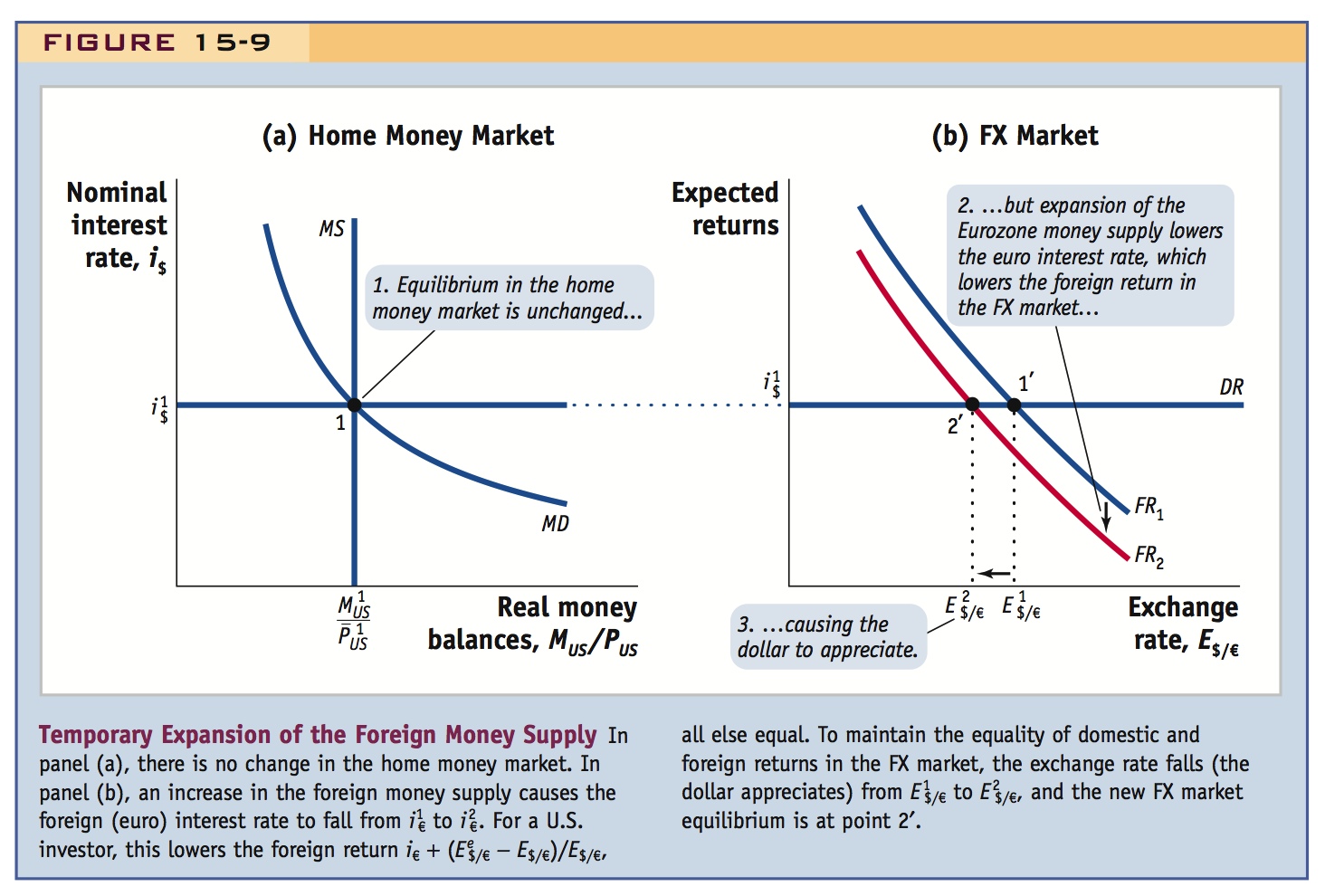
If there is a temporary increase in MEUR, the European interest rate falls. FR shifts down: capital flows to the U.S., so the dollar appreciates.
Say that we are ready to put it all together.
To simplify the graphical presentation of the asset approach, we focus on conditions in the home economy; a similar approach can be used for the foreign economy. For illustration we again assume that Home is the United States and Foreign is Europe meaning the Eurozone.
The Asset Approach to Exchange Rates: Graphical Solution
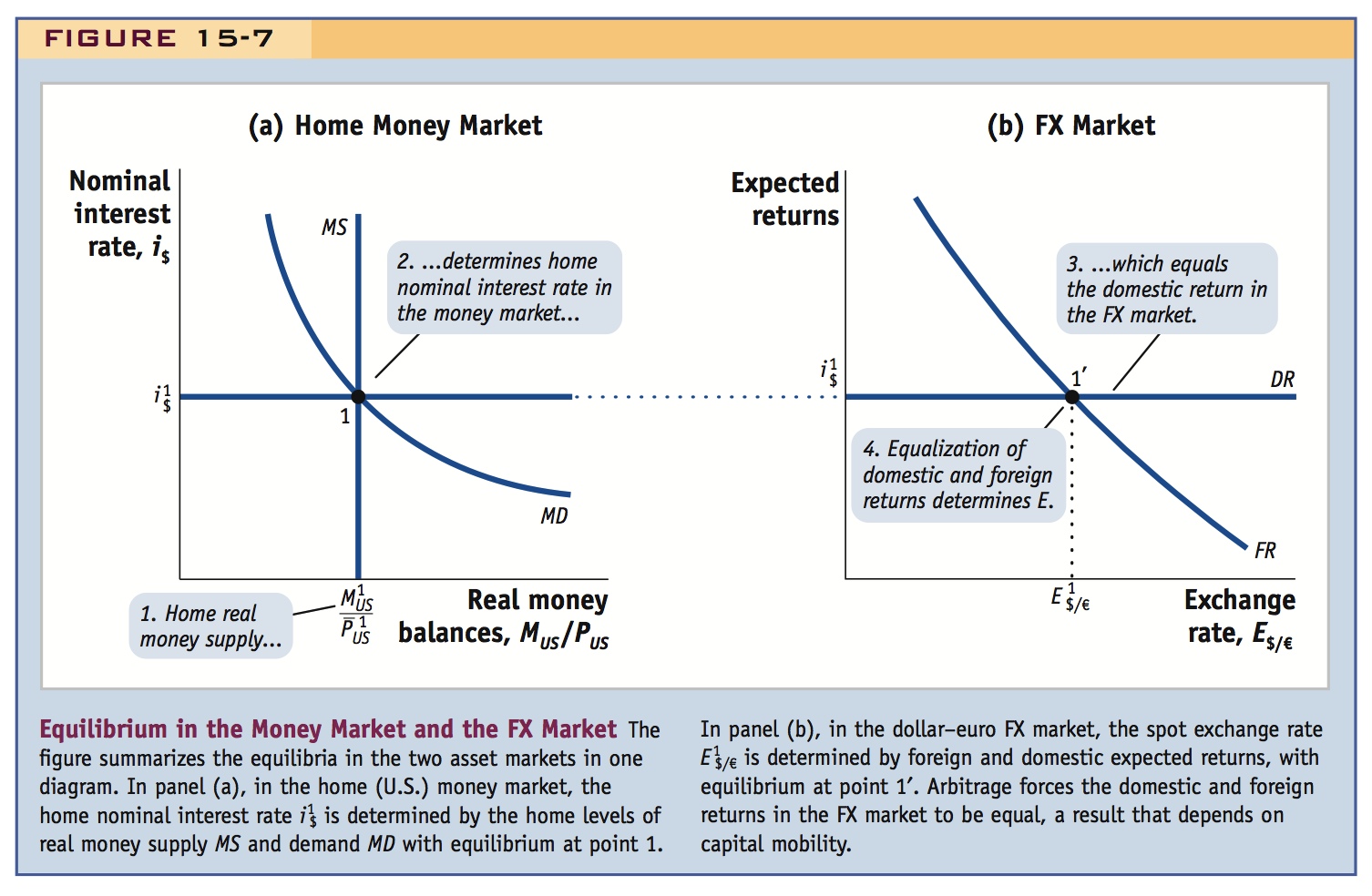
Figure 15-7 shows two markets: panel (a) shows the home money market (for the United States), and panel (b) shows the FX market diagram (for the dollar–euro market). This figure summarizes the asset approach in the short run.

The U.S. Money Market Panel (a) depicts equilibrium in the U.S. money market. The horizontal axis shows the quantity of U.S. real money balances demanded or supplied, MUS/PUS. The vertical axis shows the U.S. nominal interest rate i$. Two relationships are shown:
- The vertical line MS represents the U.S. real money supply. The line is vertical because (i) the nominal U.S. money supply MUS is treated as exogenous (known), because it is set by the home central bank, and (ii) the U.S. price level
 is treated as exogenous (known) in the short run because prices are sticky.
 - The curve MD on the diagram represents the U.S. demand for real money balances, L(i$)YUS. It slopes down because, when the home nominal interest rate i$ rises, the opportunity cost of holding money increases, and demand falls. For now, we also assume that the U.S. real income level YUS is exogenous (given) and fixed in the short run.
In equilibrium, money demand equals money supply, the quantity of real money demanded and supplied is  , and the nominal interest rate is
  (point 1).
The Market for Foreign Exchange Panel (b) depicts equilibrium in the FX market. The horizontal axis shows the spot exchange rate, E$/€. The vertical axis shows U.S. dollar returns on home and foreign deposits. Two relationships are shown:
- The downward-sloping foreign return curve FR shows the relationship between the exchange rate and the expected dollar rate of return on foreign deposits
 . The European interest rate i€ is treated as exogenous (given); it is determined in the European money market, which is not shown in this figure. The expected future exchange rate
  is treated as exogenous (given); it is determined by a forecast obtained from the long-run model we developed in the previous chapter.
 - The horizontal domestic return line DR shows the dollar rate of return on U.S. deposits, which is the U.S. nominal interest rate i$. It is horizontal at
 because this is the U.S. interest rate determined in the home money market in panel (a), and it is the same regardless of the spot exchange rate.
127
In equilibrium, foreign and domestic returns are equal (uncovered interest parity holds) and the FX market is in equilibrium at point 1′.
Because UIP wouldn't hold
Capital Mobility Is Crucial We assume that the FX market is subject to the arbitrage forces we have studied and that uncovered interest parity will hold. But this is true only if there are no capital controls: as long as capital can move freely between home and foreign capital markets, domestic and foreign returns will be equalized. Our assumption that DR equals FR depends on capital mobility. If capital controls are imposed, there is no arbitrage and no reason why DR has to equal FR.
Once again, express this as a problem in predicting how changes in exogenous things affect endogenous things. Have them identify each: There two endogenous variables, i and E, and four exogenous variables, M, Y, i*, and (for now) Ee.
Depict this by adding a row of exogenous things at the top of Figure 15-5.
Putting the Model to Work With this graphical apparatus in place, it is relatively straightforward to solve for the exchange rate given knowledge of all the known (exogenous) variables we have just specified.
To solve for the exchange rate, we start in the home money market in panel (a) on the horizontal axis, at the level of real money supply  ; we trace upward along MS to MD at point 1, to find the current home interest rate
  . We then trace right and move across from the home money market to the FX market in panel (b), since the home interest rate is the same as domestic return DR in the FX market. We eventually meet the FR curve at point 1′. We then trace down and read off the equilibrium exchange rate
  .
.
Perhaps assign this as a homework assignment. They will need to do comparative static exercises for changes in foreign M and Y.
Our graphical treatment shows that solving the model is as simple as tracing a path around the diagrams. While we gain in simplicity, we also lose some generality because one market, the foreign money market, has been left out of the analysis. However, the same analysis also applies to the foreign country. As a quick check that you understand the logic of the asset approach to exchange rates, you might try to construct the equivalent of Figure 15-7 under the assumption that Europe is Home and the United States is the Foreign. (Hint: In the FX market, you will need to treat the home [European] expected future exchange rate  and the foreign [U.S.] interest rate i$ as given. Take care with the currency units of every variable when making the switch.)
Short-Run Policy Analysis
The graphical exposition in Figure 15-7 shows how the asset approach works to determine the exchange rate. This approach can be used to analyze the impacts of economic policy or other shocks to the economy.
Emphasize that temporary shocks won't change prices or expectations.
The most straightforward shocks we can analyze are temporary shocks because they affect only the current state of the money and foreign exchange markets and do not affect expectations about the future. In this section, we use the model to see what happens when there is a temporary, short-run increase in the money supply by the central bank.
A Temporary Shock to the Home Money Supply We take the model of Figure 15-7 and assume that, apart from the home money supply, all exogenous variables remain unchanged and fixed at the same level. Thus, foreign money supply, home and foreign real income and price levels, and the expected future exchange rate are all fixed.
The initial state of all markets is shown in Figure 15-8. The home money market is in equilibrium at point 1 where home money supply MS and money demand MD are equal at the home nominal interest rate  . The foreign exchange market is in equilibrium at point 1′, where domestic return DR equals foreign return FR, where
  , and the spot exchange rate is
  .
.

128
Suppose the U.S. money supply is increased temporarily from  to
to  . Under the assumption of sticky prices,
  does not change, so the U.S. real money supply will increase to
  , and the real money supply curve shifts from MS1 MS2 in panel (a). U.S. real money demand is unchanged, so the money market equilibrium shifts from point 1 to point 2 and the nominal interest rate falls from
  to
to  . The expansion of the U.S. money supply causes the U.S. nominal interest rate to fall.
A temporary monetary policy shock leaves the long-run expected exchange rate  unchanged. Assuming all else equal, European monetary policy is also unchanged, and the euro interest rate remains fixed at i€. If
  and i€ are unchanged, then the foreign return FR curve in panel (b) is unchanged and the new FX market equilibrium is at point 2′. The lower domestic return
  is matched by a lower foreign return. The foreign return is lower because the U.S. dollar has depreciated from
  to
to  .
.
Here again, students seem to like a flow chart showing the linkages: M increases -> i falls -> demand for dollar deposits falls (and demand for euro deposits increases) -> demand for $ falls -> E increases. Relate these linkages to shifts in, and movements along, the appropriate curves above.
The result is intuitive, and we have seen each of the steps previously. We now just put them all together: a home monetary expansion lowers the home nominal interest rate, which is also the domestic return in the forex market. This makes foreign deposits more attractive and makes traders wish to sell home deposits and buy foreign deposits. This, in turn, makes the home exchange rate increase (depreciate). However, this depreciation makes foreign deposits less attractive (all else equal). Eventually, the equality of foreign and domestic returns is restored, uncovered interest parity holds again, and the foreign exchange market reaches a new short-run equilibrium.
129
Ditto
A Temporary Shock to the Foreign Money Supply We now repeat the previous analysis for a shock to the foreign money supply. All other exogenous variables remain unchanged and fixed at their initial levels. Thus, home money supply, home and foreign real income and price levels, and the expected future exchange rate are all fixed. The initial state of all markets is shown in Figure 15-9: the home money market is in equilibrium at point 1 and the FX market is in equilibrium at point 2.

Let’s see what happens when the foreign money supply increases temporarily. Because changes in the foreign money supply have no effect on the home money market in panel (a), equilibrium remains at point 1 and the home nominal interest rate stays at  .
.
The shock is temporary, so long-run expectations are unchanged, and the expected exchange rate  stays fixed in panel (b). However, because the foreign money supply has expanded temporarily, the euro interest rate falls from
  to
to  . Foreign returns are diminished, all else equal, by a fall in euro interest rates, so the foreign return curve FR shifts downward from FR1 to FR2. On the horizontal axis in panel (b), we can see that at the new FX market equilibrium (point 2′) the home exchange rate has decreased (the U.S. dollar has appreciated) from
  to
to  .
.
This result is also intuitive. A foreign monetary expansion lowers the foreign nominal interest rate, which lowers the foreign return in the forex market. This makes foreign deposits less attractive and makes traders wish to buy home deposits and sell foreign deposits. This, in turn, makes the home exchange rate decrease (appreciate). However, this appreciation makes foreign deposits more attractive (all else equal). Eventually, the equality of foreign and domestic returns is restored, uncovered interest parity holds again, and the foreign exchange market reaches a new short-run equilibrium.
130
Also do comparative static exercises for domestic and foreign incomes. Emphasize that faster growing countries should have appreciating currencies.
In addition, consider an exogenous increase in Ee. Emphasize that current spot rates can change even if current (or even expected future) fundamentals have not changed.
To ensure you have grasped the model fully, you might try two exercises. First, derive the predictions of the model for temporary contractions in the home or foreign money supplies. Second, go back to the version of Figure 15-7 that you constructed from the European perspective and generate predictions using that version of the model, first for a temporary expansion of the money supply in Europe and then for a temporary expansion in the United States. Do you get the same answers?
This is a nice example to use.
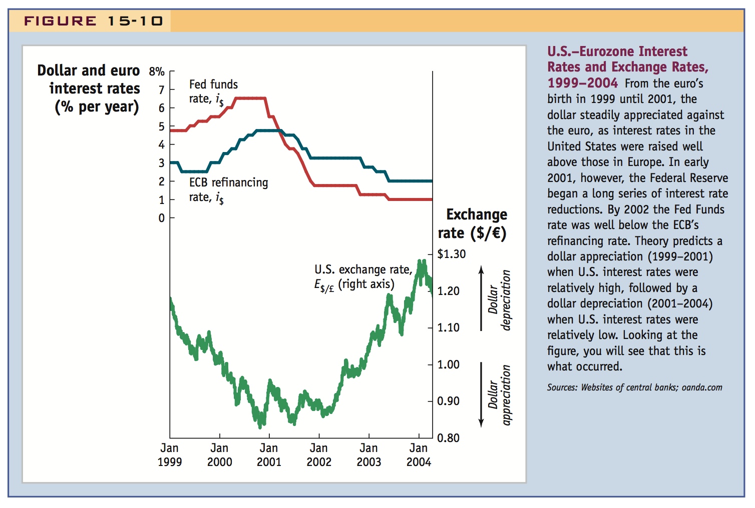
From 1999 to 2001 both the Fed and ECB raised interest rates, but the ECB was more restrained in doing so. As the model predicts, the dollar appreciated. After 2001 the Fed lowered interest rates aggressively, so the dollar depreciated.
The Rise and Fall of the Dollar, 1999–2004
In the 1990s, many developed countries adopted monetary policies that established clear, long-run nominal anchors. The European Central Bank, for example, adopted an explicit inflation target. The Federal Reserve in the United States operated with a more implicit target, but nonetheless could claim to have a credible anchor, too.
The Fisher effect tells us that nominal anchoring of this kind ought to keep nominal interest rate differentials between the United States and the Eurozone roughly constant in the long run. But in the short run, this constraint does not apply, so central banks have some freedom to temporarily change their monetary policies. In the years 2000 to 2004, such flexibility was put to use and interest rates in the United States and Europe followed very different tracks.
In later chapters, we study in more detail why central banks alter monetary policy in the short run, but for now we focus on how such changes affect exchange rates. As Figure 15-10 shows, the Fed raised interest rates from 1999 to 2001 faster than the ECB (the Fed was more worried about the U.S. economy “overheating” with higher inflation). In this period of global economic boom, the ECB’s policy also tightened over time, as measured by changes in the Euro interest rate—the refinancing rate set by the ECB. But the changes were more restrained and slower in coming.
As Figure 15-10 also shows, the Fed then lowered interest rates aggressively from 2001 to 2004, with rates falling as low as 1% in 2003 to 2004 (the U.S. economy had slowed after the boom and the Fed hoped that lower interest rates would avert a recession; the terrorist attacks of September 11, 2001, led to fears of a more serious economic setback and encouraged further monetary easing). The ECB also acted similarly to lower interest rates, but again the ECB did not move rates as far or as fast as the Fed.

As a result, the ECB’s interest rate, previously lower than the Fed’s rate, was soon higher than the U.S. rate in 2001 and remained higher through 2004. Investors most likely viewed these policy changes as a temporary shift in monetary policy in both countries. Hence, they might be considered as an example of temporary monetary policy shocks. Do our model’s predictions accord well with reality?
Up until 2001, the policy of higher rates in the United States could be seen as a temporary home monetary contraction (relative to foreign), and our model would predict a dollar appreciation in the short run. After 2001 the aggressive reductions in U.S. interest rates could be seen as a temporary home monetary expansion (relative to foreign), and our model predicts a dollar depreciation in the short run. Looking at the path of the dollar–euro exchange rate in the figure, we can see that the model accords well with reality.
131