Appendix To Chapter 17

In reality, home and foreign incomes will not have a perfect inverse correlation as we have assumed in the text. Let us generalize a bit more for our two countries, and focus on capital income.

A More General Case Suppose the shocks to capital income are a and b, for countries A and B, respectively, and that these take a random value each period. The common shock is the average shock in the two countries: . In the chapter, we assumed the average shock was zero, so the shocks were equal and opposite. In the real world, however, this need not be the case.

We can define the A-specific shock as the shock a minus the average shock: . Similarly, the B-specific shock is b minus the average shock: . These idiosyncratic shocks are nonzero as long as the A shock is not the same as the B shock, that is, as long as a is not equal to b.

By doing this algebraic manipulation, the A shock can be written as the common shock plus the A-specific shock:

Similarly, the B shock can be written as the common shock plus the B-specific shock:

We see that the country-specific shocks are the exact opposites of each other: and . The good news is that country-specific shocks are a diversifiable risk and satisfy the conditions of the simple case examined in the chapter. So the income risk they generate can be eliminated by diversification: in the world portfolio, the country-specific shocks cancel out, as we can see by adding up the last two equations.

But the common shock is . As long as this is nonzero, these shocks matter, that is, as long as the shocks are not equal and opposite, pure asymmetric country-specific shocks. The bad news is, the global shocks are an undiversifiable risk—no matter which assets you own, you get hit with the global shock, so asset trade offers no escape from these risks.

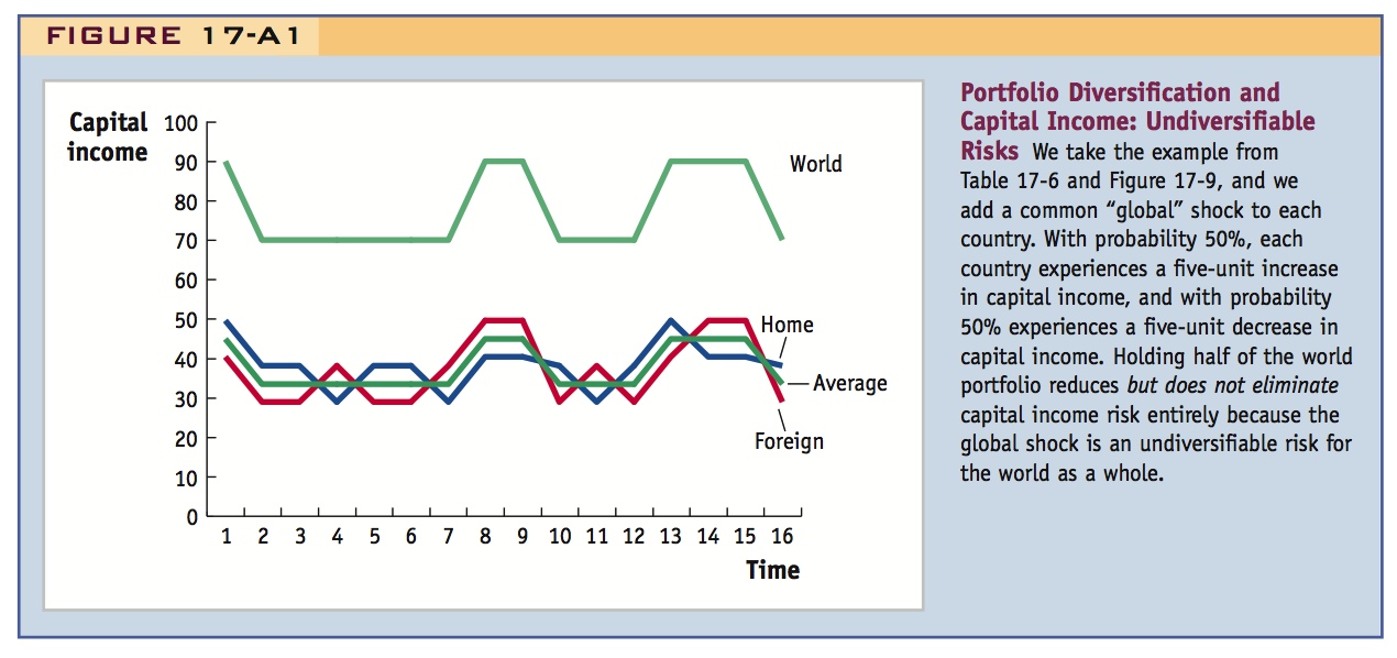
Numerical Example Figure 17-A1 (an extension of Figure 17-9) provides an illustration of the partial reduction in risk that can be achieved in this case. In Figure 17-9, each country owned 50% of the world portfolio. Thus, capital incomes in each state were as follows: in state 1, A = 36, B = 44; in state 2, A = 44, B = 36. The occurrence of states 1 and 2 was random with 50–50 odds. If A and B diversified by each holding 50% of the world portfolio, they had stable capital income of 40 every period.

Figure 17-A1, we add an extra “global” shock, which has two states, X and Y, that occur at random with 50-50 odds. However, the random X-Y shock is independent of the 1-2 shock. We suppose that when the global shock is in state X, both countries receive an extra five units of capital income. When the global shock is in state Y, both countries receive five units less of capital income.

There are now four possible states of the world: 1X, 1Y, 2X, and 2Y. Each has a 25% chance of occurring. For the four states, the capital incomes of the portfolios are as follows:

From this table, and the example shown in Figure 17-A1, we see, as expected, that in this world, holding half of the world portfolio eliminates the risk associated with fluctuations between states 1 and 2. The best that each country can do is to have an income that fluctuates between 45 (half of 90, state X) and 35 (half of 70, state Y). In state X, all income risk associated with states 1 and 2 is gone. And in state Y, all income risk associated with states 1 and 2 is gone. But nothing can be done to eliminate the risk associated with fluctuations between states X and Y.

This more general result does not overturn our basic findings. Holding a 100% home portfolio generates a volatile capital income. So does holding a 100% foreign portfolio. Holding a mix of the two lowers the volatility of capital income, at least when some of the shocks are country-specific shocks, which is always the case in the real world.