1 Demand in the Open Economy
Elaborate on this a bit more: Explain that macro models always involve the interaction of several aggregate markets, that we've already done two (money & FX) but now have one more to go.
Make sure students know what this means and that it will circumscribe the analysis.
We will need three markets: goods, money, and FX. The latter two we studied already, assuming that output was exogenous. This is appropriate in the long run. In short run, however, it can be endogenous. This section develops a short run, sticky-price model where changes in demand can affect output.
1. Preliminaries and Assumptions
Home is a small open economy. Prices  are constant; government expenditures, taxes, foreign income, and foreign interest rates are exogenous. Ignore net factor income from abroad and unilateral transfers, so that income equals GDP, Y = GDP and CA = TB. Objective: Characterize demand for Home goods and find short-run equilibrium. Demand has four components.
2. Consumption
A Keynesian consumption function defined over disposable income  with an MPC between zero and one.
3. Investment
Investment I(i) is a decreasing function of the real interest rate. There is no inflation, so i = r.
4. The Government
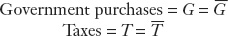
The government collects taxes  and spends
  . If
. If  there is a budget surplus; if
  there’s a deficit.
5. The Trade Balance
TB depends upon three things, the real exchange rate and disposable income in the two countries, 
a. The Role of the Real Exchange Rate: Changes in the real exchange rate  induce expenditure switching by changing the relative price of the foreign good. Normally, a real depreciation will increase exports and decrease imports, so the TB will improve.
b. The Role of Income Levels: An increase in foreign income will raise home exports; an increase in home income will increase home imports. The TB should decrease with domestic income and increase with foreign income. The marginal propensity to consume foreign imports is MPCF and that on home goods is MPCH, where MPCF + MPCH = MPC.
To understand macroeconomic fluctuations, we need to grasp how short-run disturbances affect three important markets in an economy: the goods market, the money market, and the foreign exchange (forex) market. In earlier chapters, we studied the forex market and the money market, so we will recap and apply here what we learned in those chapters. But what about the goods market? In the forex chapters, we assumed that output was fixed at a level  . We took this to be the full-employment level of output that would be expected to prevail in the long run, when all factor market prices have adjusted to ensure that all factors such as labor and capital are employed. But these assumptions about output and employment are valid only in the long run. To understand short-run fluctuations in economic activity, we now develop a short-run, sticky-price Keynesian model and show how fluctuations in demand can create fluctuations in real economic activity. To start building this model, we first make our assumptions clear and then look at how demand is defined and why it fluctuates.
Preliminaries and Assumptions
Our interest in this chapter is to study short-run fluctuations in a simplified, abstract world of two countries. Our main focus is on the home economy. We use an asterisk to denote foreign variables when we need them. For our purposes, the foreign economy can be thought of as the rest of the world. The key assumptions we make are as follows:
- Because we are examining the short run, we assume that home and foreign price levels,
 and
and  , are fixed due to price stickiness. As a result of price stickiness, expected inflation is fixed at zero,
  . If prices are fixed, all quantities can be viewed as both real and nominal quantities in the short run because there is no inflation.
 - We assume that government spending
 and taxes
  are fixed at some constant levels, which are subject to policy change.
 - We assume that conditions in the foreign economy such as foreign output
 and the foreign interest rate
  are fixed and taken as given. Our main interest is in the equilibrium and fluctuations in the home economy.
 - We assume that income Y is equivalent to output: that is, gross domestic product (GDP) equals gross national disposable income (GNDI). From our study of the national accounts, we know that the difference between the two equals net factor income from abroad plus net unilateral transfers. The analysis in this chapter could easily be extended to include these additional sources of income, but this added complexity would not offer any additional significant insights. We further assume that net factor income from abroad (NFIA) and net unilateral transfers (NUT) are zero, which implies that the current account (CA) equals the trade balance (TB); for the rest of this chapter, we shall just refer to the trade balance.
Our main objective is to understand how output (income) is determined in the home economy in the short run. As we learned from the national accounts, total expenditure or demand for home-produced goods and services is made up of four components: consumption, investment, government consumption, and the trade balance. In the following section, we see how each component is determined in the short run, and use the fact that demand must equal supply to characterize the economy’s short-run equilibrium.
Consumption
List some of the other things that might affect consumption (e.g., wealth, expectations, and interest rates), but say that for our purposes here we will focus on disposable income.
The simplest model of aggregate private consumption relates household consumption C to disposable income Yd. As we learned in Chapter 16, disposable income is the level of total pretax income Y received by households minus the taxes paid by households , so that  . Consumers tend to consume more as their disposable income rises, a relationship that can be represented by an increasing function, called the consumption function:

A typical consumption function of this form is graphed in Figure 18-1; it slopes upward because consumption increases when disposable income increases.
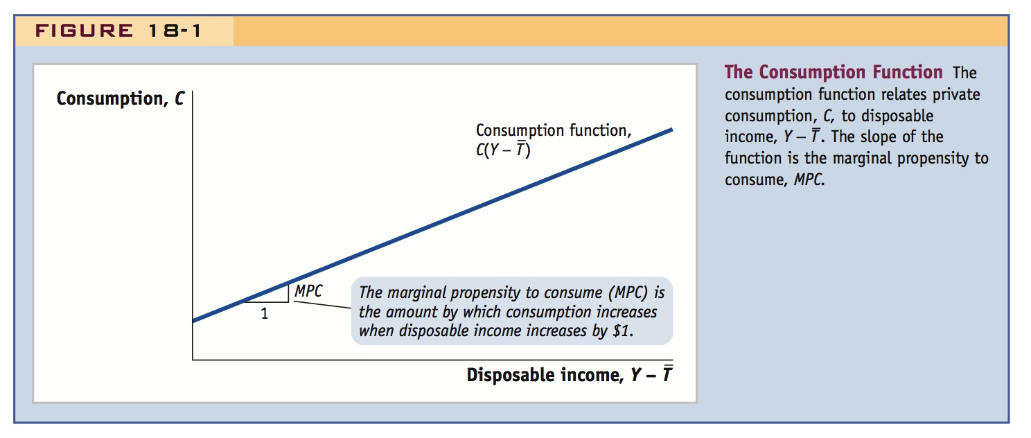
This equation is known as the Keynesian consumption function. In some economic theories, consumption smoothing is both desirable and possible. That is, in any given year consumption need not depend on income in that year, but rather on total lifetime resources (wealth). In contrast, the Keynesian consumption function assumes that private consumption expenditure is sensitive to changes in current income. This assumption seems to be a more reasonable match with reality in the short run: research shows that there is not very much consumption smoothing at the household or national level.
256
All this should be familiar to them, and so should require only a quick review.
Marginal Effects The consumption function relates the level of consumption to the level of disposable income, but we are more often interested in the response of such variables to small changes in equilibrium, due to policy shocks or other shocks. For that purpose, the slope of the consumption function is called the marginal propensity to consume (MPC), and it tells us how much of every extra $1 of disposable income received by households is spent on consumption. We generally assume that MPC is between 0 and 1: when consumers receive an extra unit of disposable income (whether it’s a euro, dollar, or yen), they will consume only part of it and save the remainder. For example, if you spend $0.75 of every extra $1 of disposable income you receive, your MPC is 0.75. The marginal propensity to save (MPS) is 1 − MPC. In this example MPS = 0.25, meaning that $0.25 of every extra $1 of disposable income is saved.
Investment
Here too, briefly discuss other things that might affect investment (expected future sales, even "animal spirits"). Possibly allude to the section on investment in the last chapter. But explain that our primary concern is the interest rate.
The simplest model of aggregate investment makes two key assumptions: firms can choose from many possible investment projects, each of which earns a different real return; and a firm will invest capital in a project only if the real returns exceed the firm’s cost of borrowing capital. The firm’s borrowing cost is the expected real interest rate re, which equals the nominal interest rate i minus the expected rate of inflation πe: re = i − πe. It is important to note that, in general, the expected real interest rate depends not only on the nominal interest rate but also on expected inflation. However, under our simplifying assumption that expected inflation is zero, the expected real interest rate equals the nominal interest rate, re = i.
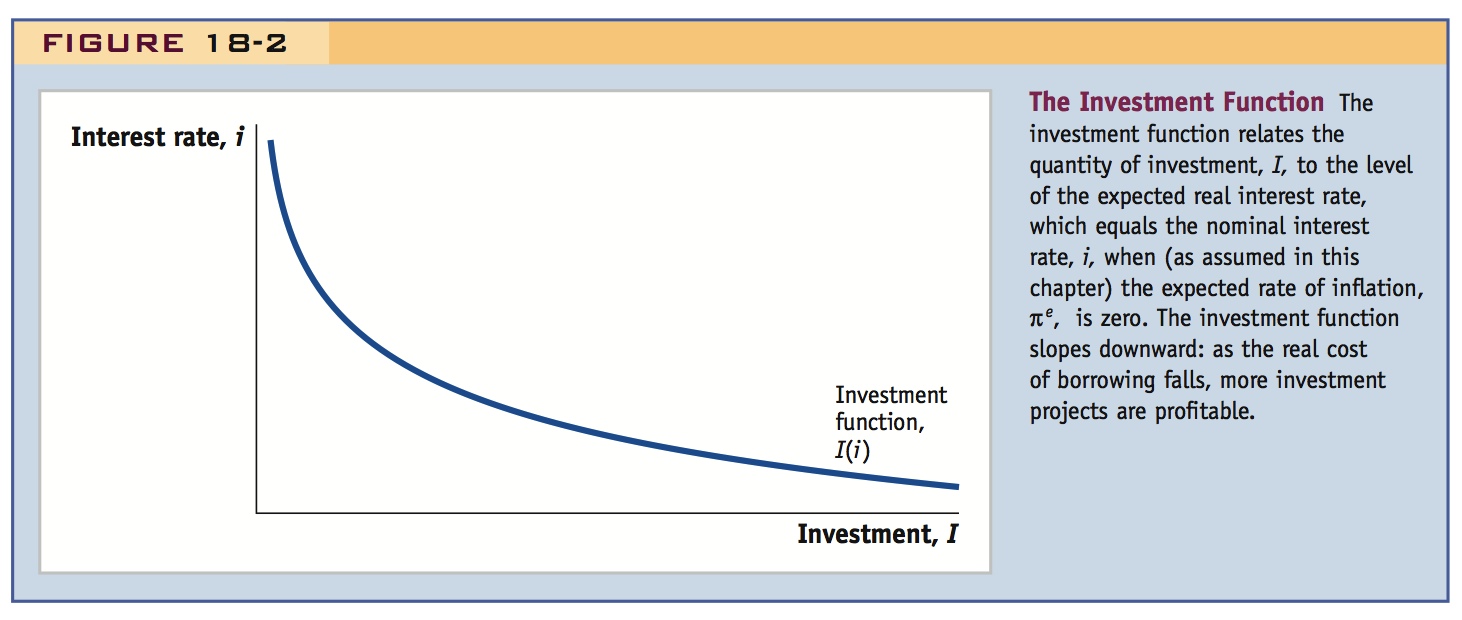
When the expected real interest rate in the economy falls, we expect more investment projects to be undertaken. For example, at a real interest rate of 10%, there may be only $1 billion worth of profitable investment projects that firms wish to undertake; but if the real interest rate falls to 5%, there may now be $2 billion worth of profitable projects. Hence, our model assumes that investment I is a decreasing function of the real interest rate; that is, investment falls as the real interest rate rises.
Investment = I = I(i)
Remember that this is true only because when expected inflation is zero, the real interest rate equals the nominal interest rate. Figure 18-2 shows a typical investment function of this type. It slopes downward because as the real interest rate falls, the quantity of investment rises.
The Government
To develop a basic model of economic activity in the short run, we assume that the government’s role is simple. It collects an amount T of taxes from private households and spends an amount G on government consumption of goods and services.
Note that the latter includes only actual spending on goods and services bought by the public sector at all levels. For example, G includes military equipment and personnel, transport and infrastructure, public universities and schools, and so forth. Excluded from this concept are the often huge sums involved in government transfer programs, such as social security, medical care, or unemployment benefit systems, that redistribute income between households. Such transfers are excluded because we assume that in the aggregate they do not generate any change in the total expenditure on goods and services; they merely change who gets to engage in the act of spending. (Transfers are like negative taxes and, as such, can be seen as a part of T.)
257
In the unlikely event that G = T exactly, government spending exactly equals taxes and we say that the government has a balanced budget. If T > G, the government is said to be running a budget surplus (of size T − G); if G > T, a budget deficit (of size G − T or, equivalently, a negative surplus of T − G).
Fiscal policy is concerned with the levels of taxes T and spending G set by the government. In this chapter, we do not study in detail why or how governments make such policy choices; we make the simple assumption that in the short run the levels of taxes and spending are set exogenously at some fixed levels, denoted by an overbar:
Policy makers may change these levels of taxes and spending at any time. We analyze the impact of such changes on the economy later in this chapter.
The Trade Balance
In the balance of payments chapter, we saw from an accounting standpoint that the trade balance (equal to exports minus imports) measures the impact of foreign trade on the demand for domestic output. To develop a model, however, we need to know what drives these flows, so in our simple model we now explore three key determinants of the trade balance: the real exchange rate, the level of home income, and the level of foreign income.
The Role of the Real Exchange Rate What is the role of the real exchange rate? Recall George, the American tourist we met at the start of our study of exchange rates, who had to deal with a weaker dollar during his visits to Paris over the course of several years. If U.S. and French prices are sticky (constant in euro and U.S. dollar terms), then as the U.S. exchange rate depreciates, the prices of French goods and services became more and more expensive in dollar terms. In the end, George was ready to take a vacation in California instead. In the aggregate, when spending patterns change in response to changes in the real exchange rate, we say that there is expenditure switching from foreign purchases to domestic purchases.
258
Make sure they understand this term.
Expenditure switching is a major factor in determining the level of a country’s exports and imports. When learning about exchange rates in the long run, we saw that the real exchange rate is the price of goods and services in a foreign economy relative to the price of goods and services in the home economy. If Home’s exchange rate is E, the Home price level is (fixed in the short run), and the Foreign price level is (also fixed in the short run), then the real exchange rate q of Home is defined as  .
.
For example, suppose that the home country is the United States, and the reference basket costs $100; suppose that in Canada the same basket costs C$120 and the exchange rate is $0.90 per Canadian dollar. In the expression  , the numerator
  is the price of foreign goods converted into home currency terms, $108 = 120 × 0.90; the denominator is the home currency price of home goods, $100; the ratio of the two is the real exchange rate, q = $108/$100 = 1.08. This is the relative price of foreign goods in terms of home goods. In this case, Canadian goods are more expensive than U.S. goods.
Actually, this disguises the fact that the price per unit of imports will change with the exchange rate. It is not too much of a digression to derive the conditions under which it is true that a real depreciation will improve the trade balance (i.e., the Marshall-Lerner condition). One could also relate it to the ensuing discussion of the J-curve.
Also emphasize, as the article below does, that depreciation stimulates domestic demand stealing it from abroad.
A rise in the home real exchange rate (a real depreciation) signifies that foreign goods have become more expensive relative to home goods. As the real exchange rate rises, both home and foreign consumers will respond by expenditure switching: the home country will import less (as home consumers switch to buying home goods) and export more (as foreign consumers switch to buying home goods). These concepts are often seen in economic debates and news coverage (see Headlines: Oh! What a Lovely Currency War and Headlines: The Curry Trade) and they provide us with the following insight:
- We expect the trade balance of the home country to be an increasing function of the home country’s real exchange rate. That is, as the home country’s real exchange rate rises (depreciates), it will export more and import less, and the trade balance rises.
The Role of Income Levels The other determinant of the trade balance we might wish to consider is the income level in each country. As we argued earlier in our discussion of the consumption function, when domestic disposable income increases, consumers tend to spend more on all forms of consumption, including consumption of foreign goods. These arguments provide a second insight:
Go ahead and define the MPCF at this point
- We expect an increase in home income to be associated with an increase in home imports and a fall in the home country’s trade balance.
Symmetrically, from the rest of the world’s standpoint, an increase in rest of the world income ought to be associated with an increase in rest of the world spending on home goods, resulting in an increase in home exports. This is our third insight:
- We expect an increase in rest of the world income to be associated with an increase in home exports and a rise in the home country’s trade balance.
Combining the three insights above, we can write the trade balance as a function of three variables: the real exchange rate, home disposable income, and rest of the world disposable income:
259
Describes the irritation of export-driven countries like Brazil and South Korea at policies to weaken the value of the won and the yen.
Oh! What a Lovely Currency War
In September 2010, the finance minister of Brazil accused other countries of starting a “currency war” by pursuing policies that made Brazil’s currency, the real, strengthen against its trading partners, thus harming the competitiveness of his country’s exports and pushing Brazil’s trade balance toward deficit. By 2013 fears about such policies were being expressed by more and more policymakers around the globe.
“Devaluing a currency,” one senior Federal Reserve official once told me, “is like peeing in bed. It feels good at first, but pretty soon it becomes a real mess.”
In recent times, foreign-exchange incontinence appears to have been the policy of choice in capitals from Beijing to Washington, via Tokyo. The resulting mess has led to warnings of a global “currency war” that could spiral into protectionism.
The roll call of forex Cassandras reads like a who’s who of global finance and politics: German leader Angela Merkel, Federal Reserve Bank of St. Louis President James Bullard, Bundesbank President Jens Weidmann and Mervyn King, the outgoing governor of the Bank of England. And the list goes on…
Currency wars have been a staple of modern finance ever since the collapse of the Bretton Woods system of fixed exchange rates in the early 1970s. As Marc Chandler, global head of currency strategy at Brown Brothers Harriman & Co., says: “Most governments believe that their currencies are too important to be left to the markets.” So policy makers have often tried to manipulate the value of their currencies by intervening in the markets.
In recent years, China stands out as the country that has done the most to keep its currency weak in order to boost exports. But it isn’t alone. China’s efforts have sparked what Fred Bergsten, senior fellow at the Peterson Institute for International Economics, calls “emulation and retaliation.”
At their worst, these periodic crosscurrents of intervention have led to “beggarthy-neighbor” policies—self-defeating attempts to improve one country’s economy at the expense of everybody else’s….
As developed countries like Japan and the U.S. try to kick-start their sluggish economies with ultralow interest rates and binges of money-printing, they are putting downward pressure on their currencies. The loose monetary policies are primarily aimed at stimulating domestic demand. But their effects spill over into the currency world.
Since the end of November, when it became clear that Shinzo Abe and his agenda of growth-at-all-costs would win Japan’s elections, the yen has lost more than 10% against the dollar and some 15% against the euro.
These moves are angering export-driven countries such as Brazil and South Korea. But they also are stirring the pot in Europe. The euro zone has largely sat out this round of monetary stimulus and now finds itself in the invidious position of having a contracting economy and a rising currency—making Thursday’s meeting of the European Central Bank a must-watch event.
The dirty secret is that using monetary policy to weaken a currency, whether voluntarily or not, is a shortcut to avoid unpopular decisions on fiscal and budgetary issues.
Breakdowns of the global foreign-exchange system have occurred with drastic regularity, but that doesn’t mean this currency war will end in tears.
For a start, common sense could prevail, putting an end to the dangerous game of beggar (and blame) thy neighbor. After all, the International Monetary Fund was set up to prevent such races to the bottom, and should try to broker a truce among forex combatants.
If that sounds naive, consider the possibility that this huge bout of monetary stimulus will succeed in engendering a solid recovery driven by domestic demand. Or that fiscal policy will finally be put to work.
Either outcome would take away a big incentive for competitive devaluations and prompt governments to bolster their currencies to avoid stoking inflation.
Growth cures a lot of ills. Even forex incontinence.
Source: Excerpted from Francesco Guerrera, “Currency War Has Started,” The Wall Street Journal, February 4, 2013. Reprinted with permission of The Wall Street Journal, Copyright © 2013 Dow Jones & Company, Inc. All Rights Reserved Worldwide.
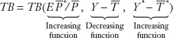
Figure 18-3 shows the relationship between the trade balance and the real exchange rate for the home country, all else equal—that is, holding home and foreign disposable income fixed. The trade balance is an increasing function of the real exchange rate  . Thus, the relationship shown in Figure 18-3 is upward sloping. The reason is that an increase in the real exchange rate (a real depreciation) increases TB by raising exports and lowering imports, implying a movement along the curve drawn.
Yes, assuming the Marshall-Lerner condition holds.
260
This is also a neat example for class discussion because it makes the effects of the change in exchange rate concrete.
Describes how the appreciation of the euro relative to the pound caused Britons living in France to order food—even French specialties—from English supermarkets.
The Curry Trade
In 2009, a dramatic weakening of the pound against the euro sparked an unlikely boom in cross-Channel grocery deliveries.
If carrying coals to Newcastle is judged a pointless exercise, then importing croissants, baguettes and bottles of claret into France might seem even more absurd. But, due to the strength of the euro against the pound, hundreds of Britons living in France are now using the internet to order their food, including many French specialties, from British supermarkets.
Simon Goodenough, the director of Sterling Shopping, a delivery firm based in Brackley, Northamptonshire, says his company has 2,500 British customers in France and is running five delivery vans full of food to France each week.
“We deliver food from Waitrose, Sainsbury’s and Marks and Spencer, but by far the biggest is Asda,” said Goodenough “…We sit in our depot sometimes looking at the things people have bought and just laugh at the craziness of it all. We have seen croissants and baguettes in people’s shopping bags. And we have delivered bottles of Bergerac wine bought from Sainsbury’s to a customer in Bergerac. We even have a few French customers who have now heard about what we do. They love things like curries and tacos, which they just can’t get in France.”…
Goodenough said many of his company’s British customers hold pensions or savings in sterling rather than euros: “They have seen a 30% drop in their spending power over the past 18 months.”
John Steventon owns La Maison Removals, a delivery company based in Rayleigh, Essex. It takes food from its warehouse to about 1,000 British customers in central France.
“We just can’t cope with demand at the moment,” he said…. “We found that friends in France were asking us to bring over British food for them so we just thought it made sense to set up a food delivery service…. The savings for buying food, in particular, are amazing due to the strength of the euro. Customers tell us that for every £100 they would spend in France buying food, they save £30 buying through us, even with our 15% commission. A lot of people are using us to get things they really miss, such as bacon and sausages.”
Nikki Bundy, 41, has lived near Périgueux in the Dordogne with her family for four years…. “It’s just so much cheaper for us to buy our food this way…. The food in France is lovely, but you can come out of a supermarket here with just two carrier bags having spent €100. I still try and buy my fresh fruit and veg in France, but most other things I now buy from Asda.”
Source: Excerpted from Leo Hickman, “Expat Orders for British Supermarket Food Surge on Strength of euro,” The Guardian, June 9, 2010. Copyright Guardian News & Media Ltd 2010.
261
The effect of the real exchange rate on the trade balance is now clear. What about the effects of changes in output? Figure 18-3 also shows the impact of an increase in home output on the trade balance. At any level of the real exchange rate, an increase in home output leads to more spending on imports, lowering the trade balance. This change would be represented as a downward shift in the trade balance curve, that is, a reduction in TB for a given level of  .
.
Marginal Effects Once More The impact of changes in output on the trade balance can also be thought of in terms of the marginal propensity to consume. Suppose home output (which equals home income, because of the assumptions we’ve made) rises by an amount ΔY = $1 and that, all else equal, this leads to an increase in home imports of ΔIM = $MPCF, where MPCF > 0. We refer to MPCF as the marginal propensity to consume foreign imports. For example, if MPCF = 0.1, this means that out of every additional $1 of income, $0.10 are spent on imports.
How does MPCF relate to the MPC seen earlier? After a $1 rise in income, any additional goods consumed have to come from somewhere, home or abroad. The fraction $MPC of the additional $1 spent on all consumption must equal the sum of the incremental spending on home goods plus incremental spending on foreign goods. Let MPCH > 0 be the marginal propensity to consume home goods. By assumption, MPC = MPCH + MPCF. For example, if MPCF = 0.10 and MPCH = 0.65, then MPC = 0.75; for every extra dollar of disposable income, home consumers spend 75 cents—10 cents on imported foreign goods and 65 cents on home goods—and they save 25 cents.1
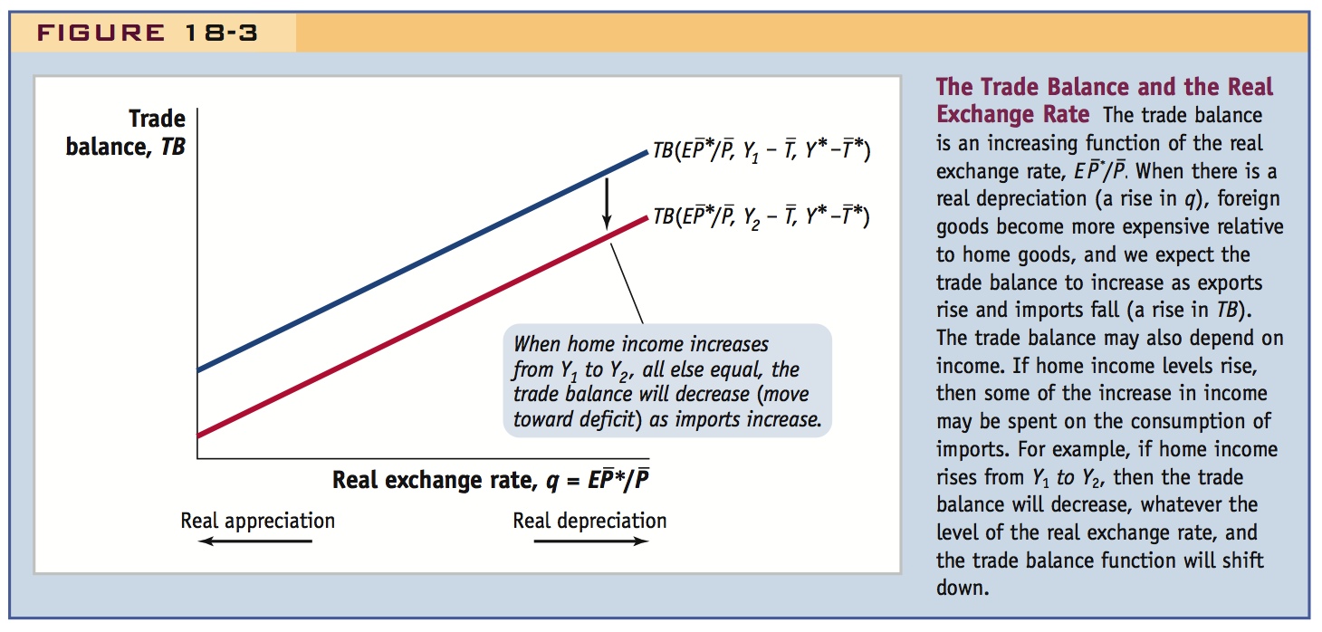
From 1975-2012, the U.S. TB was positively correlated with its multilateral real exchange rate, but not perfectly. Why not? (1) Imports and export react to exchange rate changes with lags; (2) other things may have been changing at the same time.
The Trade Balance and the Real Exchange Rate
Our theory assumes that the trade balance increases when the real exchange rate rises. Is there evidence to support this proposition? In Figure 18-4, we examine the evolution of the U.S. trade balance (as a share of GDP) in recent years as compared with the U.S. real exchange rate with the rest of the world.
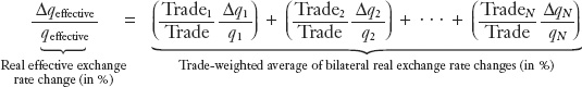
By considering the home country to be the United States and the foreign “country” to be the rest of the world, we cannot use data on the bilateral real exchange rate q for any individual foreign country. We need a composite or weighted-average measure of the price of goods in all foreign countries relative to the price of U.S. goods. To accomplish this, economists construct multilateral measures of real exchange rate movement.
The most common weighting scheme uses a weight equal to that country’s share in the home country’s trade. If there are N foreign countries, we can write home’s total trade as the sum of its trade with each foreign country: Trade = Trade1 + Trade2 + … + TradeN. Applying a trade weight to each bilateral real exchange rate’s percentage change, we obtain the percentage change in home’s multilateral real exchange rate or real effective exchange rate:
262
For example, if we trade 40% with country 1 and 60% with country 2, and we have a real appreciation of 10% against 1 but a real depreciation of 30% against 2, then the change in our real effective exchange rate is (40% × −10%) + (60% × 30%) = (0.4 × −0.1) + (0.6 × 0.3) = −0.04 + 0.18 = 0.14 = +14%. That is, we have experienced an effective trade-weighted real depreciation of 14%.
Figure 18-4 shows that the U.S. multilateral real exchange rate and the U.S. trade balance have been mostly positively correlated, as predicted by our model. In periods when the United States has experienced a real depreciation, the U.S. trade balance has tended to increase. Conversely, real appreciations have usually been associated with a fall in the trade balance. However, the correlation between the real exchange rate and the trade balance is not perfect. There appears to be lag between, say, a real depreciation and a rise in the trade balance (as in the mid-1980s). Why? Import and export flows may react only slowly or weakly to changes in the real exchange rate, so the trade balance can react in unexpected ways (see Side Bar: Barriers to Expenditure Switching: Pass-Through and J Curve). We can also see that the trade balance and real exchange rate did not move together as much during the years 2000 to 2008 because other factors, such as tax cuts and wartime spending, may have created extra deficit pressures that spilled over into the U.S. current account during this period.
This is a nice stylized fact to use to introduce the J curve.
263
Discusses how dollarization and euro invoicing limit the extent to which depreciation causes expenditure switching. Also discusses how lags in the response of exports and imports to depreciation can produce the J Curve.
6. Exogenous Changes in Demand
Things that will change demand, other than and : Exogenous changes in C,I, or TB.
Students find this to be an interesting digression.
Barriers to Expenditure Switching: Pass-Through and the J Curve
The basic analysis of expenditure switching in the text assumes two key mechanisms. First, we assume that a nominal depreciation causes a real depreciation and raises the price of foreign imports relative to home exports. Second, we assume that such a change in relative prices will lower imports, raise exports, and increase the trade balance. In reality, there are reasons why both mechanisms operate weakly or with a lag.
Trade Dollarization, Distribution, and Pass-Through
One assumption we made was that prices are sticky in local currency. But what if some home goods prices are set in foreign currency?
For example, let the foreign country be the United States and suppose a share d of the home-produced basket of goods is priced in U.S. dollars at a sticky dollar price  . Suppose that the remaining share, 1 − d, is priced, as before, in local currency at a sticky local currency price
  . Hence,
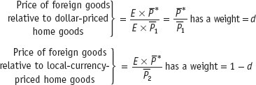
In this setup, what is the price of all foreign-produced goods relative to all home-produced goods (the real exchange rate)? It is the weighted sum of the relative prices of the two parts of the basket. Hence, we find
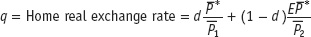
The first term with a weight d does not contain E because both numerator and denominator are dollar prices (already expressed in a common currency). Only the second term with a weight (1 − d) contains E, since the prices are in different currencies. Thus, a 1% increase in E will lead to only a (1 − d)% increase in the real exchange rate.
When d is 0, all home goods are priced in local currency and we have our basic model. A 1% rise in E causes a 1% rise in q. There is full pass-through from changes in the nominal exchange rate to changes in the real exchange rate. But as d rises, pass-through falls. If d is 0.5, then a 1% rise in E causes just a 0.5% rise in q. The real exchange rate becomes less responsive to changes in the nominal exchange rate, and this means that expenditure switching effects will be muted.
It turns out that many countries around the world conduct a large fraction of their trade in a currency other than their own, such as U.S. dollars. The most obvious examples of goods with dollar prices are the major commodities: oil, copper, wheat, and so on. In some Persian Gulf economies, a nominal depreciation of the exchange rate does almost nothing to change the price of exports (more than 90% of which is oil priced in dollars) relative to the price of imports (again, overwhelmingly priced in dollars).
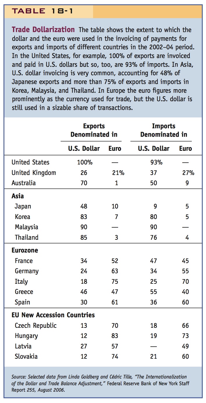
But dollar invoicing—and in Greater Europe, euro invoicing—extends around the world, as shown in Table 18-1. More than 90% of U.S. imports are priced in dollars: all else equal, a U.S. depreciation will hardly change the prices of these imports at all. Some Asian countries have trade flows that are 70% to 90% dollarized. Much of this is intra-Asian trade; if, say, a Korean supplier sells to a Japanese manufacturer, very often they conduct the trade not in yen or won, but entirely in U.S. dollars, which is the currency of neither the exporter nor the importer! The table also shows that many new EU member states in Eastern Europe have export shares largely denominated in euros.
264
Trade dollarization is not the only factor limiting pass-through in the real world. Even after an import has arrived at the port, it still has to pass through various intermediaries. The retail, wholesale, and other distribution activities all add a local currency cost or markup to the final price paid by the ultimate buyer. Suppose the markup is $100 on an import that costs $100 at the port, so the good retails for $200 in shops. Suppose a 10% depreciation of the dollar raises the port price to $110. All else equal, the retail price will rise to just $210, only a 5% increase at the point of final sale. Thus, expenditure switching by final users will be muted by the limited pass-through from port prices to final prices.
How large are these effects? A study of 76 developed and developing countries found that, over the period of one year, a 10% exchange rate depreciation resulted in a 6.5% rise in imported goods prices at the port of arrival but perhaps only a 4% rise in the retail prices of imported goods.*
The J Curve
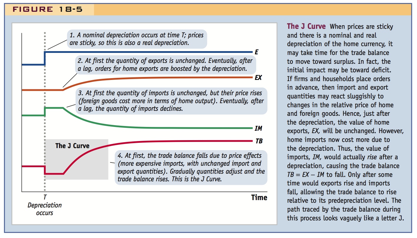
Our model of the trade balance assumes that a real depreciation improves a country’s trade balance by increasing exports and reducing imports. In reality, however, these effects may be slow to appear because orders for export and import goods are placed months in advance. Thus, at the moment of depreciation there will be no instantaneous change in export and import volumes.
What does this slow adjustment imply? Exports will continue to sell for a time in the same quantity and at the same domestic price, and so total export earnings remain fixed. What will change is the domestic price paid for the import goods. They will have become more expensive in domestic currency terms. If the same quantity of imports flows in but costs more per unit, then the home country’s total import bill will rise.
As a result, if export earnings are fixed but import expenditures are rising, the trade balance will initially fall rather than rise, as shown in Figure 18-5. Only after time passes, and export and import orders adjust to the new relative prices, will the trade balance move in the positive direction we have assumed. Because of its distinctive shape, the curve traced out by the trade balance over time in Figure 18-5 is called the J Curve. Some empirical studies find that the effects of the J Curve last up to a year after the initial depreciation. Hence, the assumption that a depreciation boosts spending on the home country’s goods may not hold in the very short run.
* Jeffrey A. Frankel, David C. Parsley, and Shang-Jin Wei, 2005, “Slow Passthrough Around the World: A New Import for Developing Countries?” National Bureau of Economic Research (NBER) Working Paper No. 11199.
265
Exogenous Changes in Demand
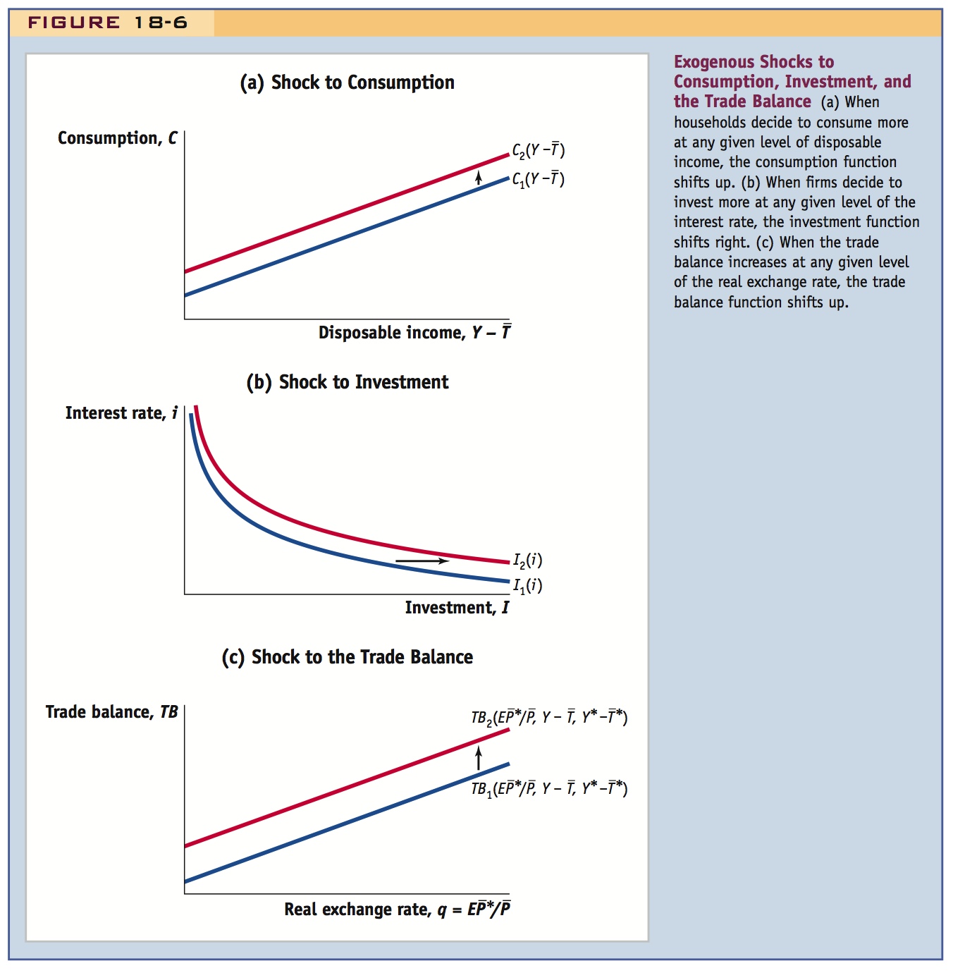
We have already treated as given, or exogenous, the changes or shocks in demand that originate in changes to government purchases or taxes. However, other exogenous changes in demand can affect consumption, investment, or the trade balance, and it is important to know how to analyze these, too. Examples of such changes are illustrated in Figure 18-6.
This is why it is useful to mention earlier that C might depend upon wealth.
Here too it would help if you had already mentioned other exogenous things of which I might be a function.
- An exogenous change in consumption. Suppose that at any given level of disposable income, consumers decide to spend more on consumption. After this shock, the consumption function would shift up as in Figure 18-6, panel (a). For example, an increase in household wealth following a stock market or housing market boom (as seen in expansions since 1990) could lead to a shift of this sort. This is a change in consumption demand unconnected to disposable income.
- An exogenous change in investment. Suppose that at any given level of the interest rate, firms decide to invest more. After this shock, the investment function would shift up as in Figure 18-6, panel (b). For example, a belief that high-technology companies had great prospects for success led to a large surge in investment in this sector in many countries in the 1990s. This is a change in investment demand unconnected to the interest rate.
- An exogenous change in the trade balance. Suppose that at any given level of the real exchange rate, export demand rises and/or import demand falls. After one of these shocks, trade balance function would shift up as in Figure 18-6, panel (c). Such a change happened in the 1980s when U.S. consumers’ tastes shifted away from the large domestic automobiles made in Detroit toward smaller fuel-efficient imported cars manufactured in Japan. This is a switch in demand away from U.S. and toward Japanese products unconnected with the real exchange rate.