2 Goods Market Equilibrium: The Keynesian Cross

We have now studied the determinants of each component of demand. We next put all the components together and show that the goods market is in equilibrium when total demand from all these components is equal to total supply.

Supply and Demand

The total aggregate supply of final goods and services is equal to total national output measured by GDP. Given our assumption that the current account equals the trade balance, gross national income Y equals GDP:

Aggregate demand, or just “demand,” consists of all the possible sources of demand for this supply of output. In the balance of payments chapter, we studied the expenditure side of the national income accounts and saw that supply is absorbed into different uses according to the national income identity. This accounting identity always holds true. But an identity is not an economic model. A model must explain how, in equilibrium, the observed demands take on their desired or planned values and still satisfy the accounting identity. How can we construct such a model?

We may write total demand for GDP as

We can substitute the formulae for consumption, investment, and the trade balance presented in the first section of this chapter into this total demand equation to obtain

Finally, in an equilibrium, demand D must equal supply Y, so from the preceding two equations we can see that the goods market equilibrium condition is

Determinants of Demand

The right-hand side of Equation (7-1) shows that many factors can affect demand: home and foreign output (Y and Y^*), home and foreign taxes (T and T^*), the home nominal interest rate (i), government spending , and the real exchange rate . Let us examine each of these in turn. We start with home output Y, and assume that all other factors remain fixed.

A rise in output Y (all else equal) will cause the right-hand side to increase. For example, suppose output increases by ΔY = $1. This change causes consumption spending C to increase by +$MPC. The change in imports will be +$MPC_F, causing the trade balance to change by −$MPC_F. So the total change in D will be $(MPC − MPC_F) = $MPC_H > 0, a positive number. This is an intuitive result: an extra $1 of output generates some spending on home goods (an amount $MPC_H), with the remainder either spent on foreign goods (an amount $MPC_F) or saved (an amount $MPS).

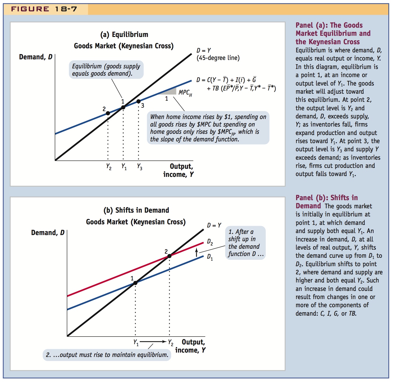
Using this result, Figure 18-7, panel (a), plots demand D, the right-hand side of Equation (7-1), as a function of income or output Y only. For the moment, we hold fixed all other determinants of D. Because D increases as Y increases, the demand function has a positive slope MPC_H, a number between 0 and 1.

Also drawn is the 45-degree line, which represents Y, the left-hand side of Equation (7-1). The 45-degree line has a slope of 1, so it is steeper than the demand function.

This diagram is often called the Keynesian cross. It depicts the goods market equilibrium: the goods market is in equilibrium at point 1 where the two lines intersect, for that is the unique point where D = Y. This corresponds to an income or output level of Y₁.

Why does the goods market adjust to an equilibrium at this point? To the right of point 1, output tends to fall; to the left of point 1, output tends to rise. Why? At point 2, the output level is Y₂ and demand D exceeds supply Y; as inventories fall, firms expand production and output rises toward Y₁. At point 3, the output level is Y₃ and supply Y exceeds demand; as inventories rise, firms cut production and output falls toward Y₁. Only at point 1 are firms in an equilibrium in which production levels are stable in the short run.

Note the crucial assumptions in this model are that prices are fixed and firms are willing to adjust their production and employment to meet whatever the desired level of demand happens to be. These assumptions may be realistic in the short run, but they do not apply in the long run, when prices can adjust and output and employment are determined by the economy’s ability to fully employ its technology and resources.

Factors That Shift the Demand Curve

The Keynesian cross also allows us to examine the impact of the other factors in Equation (7-1) on goods market equilibrium. Let’s look at four important cases:

• A change in government spending. An exogenous rise in government purchases (all else equal) increases demand at every level of output, as seen in Equation (7-1). More government purchases directly add to the total demand in the economy. This change causes an upward shift in the demand function D, as in Figure 18-7, panel (b). Goods market equilibrium shifts from point 1 to point 2, to an output level Y₂.

The lesson: any exogenous change in G (due to changes in the government budget) will cause the demand curve to shift.

• A change in taxes (or other factors affecting consumption). A fall in taxes (all else equal) increases disposable income. When consumers have more disposable income, they spend more on consumption. This change raises demand at every level of output Y, because C increases as disposable income increases. This is seen in Equation (7-1) and in Figure 18-7, panel (a). Thus, a fall in taxes shifts the demand function upward from D₁ to D₂, as shown again in Figure 18-7, panel (b). The increase in D causes the goods market equilibrium to shift from point 1 to point 2, and output rises to Y₂.

The lesson: any exogenous change in C (due to changes in taxes, tastes, etc.) will cause the demand curve to shift.

• A change in the home interest rate (or other factors affecting investment). A fall in the interest rate i (all else equal) will lead to an increase in I, as firms find it profitable to engage in more investment projects, and spend more. This change leads to an increase in demand D at every level of output Y. The demand function D shifts upward, as seen in Figure 18-7, panel (b). The increase in demand causes the goods market equilibrium to shift from point 1 to point 2, and output rises to Y₂.

The lesson: any exogenous change in I (due to changes in interest rates, the expected profitability of investment, changes in tax policy, etc.) will cause the demand curve to shift.

• A change in the home exchange rate. A rise in the nominal exchange rate E (all else equal) implies a rise in the real exchange rate EP^*/P (due to sticky prices). This is a real depreciation, and through its effects on the trade balance TB via expenditure switching, it will increase demand D at any given level of home output Y. For example, spending switches from foreign goods to American goods when the U.S. dollar depreciates. This change causes the demand function D to shift up, as seen yet again in Figure 18-7, panel (b).

The lesson: any change in the exchange rate will cause the demand curve to shift.

• A change in the home or foreign price level. If prices are flexible, then a rise in foreign prices or a fall in domestic prices causes a home real depreciation, raising . This real depreciation causes TB to rise and, all else equal, it will increase demand D at any given level of home output Y. For example, spending switches from foreign goods to American goods when the U.S. prices fall. This change causes the demand function D to shift up, as seen yet again in Figure 18-7, panel (b).

The lesson: any change in P^* or P will cause the demand curve to shift.

Summary

An increase in output Y causes a move along the demand curve (and similarly for a decrease). But any increase in demand that is not due to a change in output Y will instead cause the demand curve itself to shift upward in the Keynesian cross diagram, as in Figure 18-7, panel (b). Similarly, any contraction in demand not due to output changes will cause the demand function to shift downward.

To conclude, the main factors that shift the demand curve out are as follows:

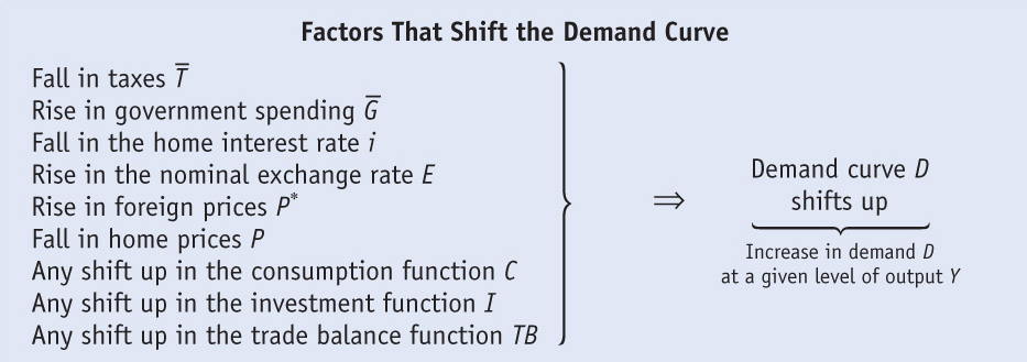
The opposite changes lead to a decrease in demand and shift the demand curve in.