1 Exchange Rate Regime Choice: Key Issues
Use the models developed, in conjunction with other theory and evidence, to assess the pros and cons of fixed and flexible rates.
Say that fixed rates have costs and benefits. To clarify an important cost we will look at this example; this is a long, interesting detour, but tell the students that we will return to benefits later.
This is a classic example that students find interesting as an historical episode. But it also highlights the consequences of asymmetric shocks under fixed rates.
In previous chapters, we have examined the workings of the economy under fixed and floating exchange rates. One advantage of understanding the workings of these regimes in such detail is that we are now in a position to address a perennially important macroeconomic policy question: What is the best exchange rate regime choice for a given country at a given time? In this section, we explore the pros and cons of fixed and floating exchange rates by combining the models we have developed with additional theory and evidence. We begin with an application about Germany and Britain in the early 1990s. This story highlights the choices policy makers face as they choose between fixed exchange rates (pegs) and floating exchange rates (floats).
As an example, consider Britain’s decision to abandon a peg in 1992. Britain joined the EU in the 1970s. EU countries saw fixing rates (through the ERM) as a step towards a single market and a single currency. In practice, the Bundesbank set its own monetary policy and other countries pegged to the DM. Britain joined the ERM in 1990, losing control of its monetary policy.
a. A Shock in Germany
German reunification in 1990 required increased government expenditures. This started to raise German interest rates. Meanwhile the Bundesbank reduced the money supply to keep the economy from overheating. This raised German interest rates even more.
b. Choices for the Other ERM Countries
The increase in German interest rates put pressure on the pound to depreciate, improving the TB and stimulating British aggregate expenditures. Policy choices:
c. Choice 1: Float and Prosper?
Abandon the peg and let the pound depreciate. Income would increase and TB improve.
d. Choice 2: Peg and Suffer?
Maintain the peg by reducing the money supply and making interest rates increase. Britain would slip into a recession.
e. What Happened Next?
In September 1992, Britain opts for Choice 1, and dropped out of the ERM. It lowered its interest rates and let the pound depreciate. France opted for Choice 2, and stayed in the ERM. This forced it to raise interest rates and suffered slower growth.
1. Key Factors in Exchange Rate Regime Choice: Integration and Similarity
The benefit of a fixed rate is that it can lower transaction costs and enhance trade. However, the 1992 episode highlights the danger of the potential cost of a fixed rate when countries face asymmetric macroeconomic shocks.
2. Economic Integration and the Gains in Efficiency
Having a fixed exchange might reduce transaction costs. This would encourage integration, and raise the volume of trade. The lesson: As integration increases, the efficiency benefits of having a fixed exchange rate increase.
3. Economic Similarity and the Costs of Asymmetric Shocks
The example of Britain and Germany demonstrates the costs of having fixed rates when countries face asymmetric macroeconomic shocks. If shocks are symmetric, this is not a problem: If both Britain and Germany were to face an exogenous increase in demand, they both could respond by raising interest rates, and not change the peg. The lesson: If countries face more symmetric shocks and fewer asymmetric ones, then the economic costs of fixing the exchange rate are lower.
4. Simple Criteria for Fixed Exchange Rate
As integration rises, the efficiency benefits of fixing increase. As symmetry rises, the stability costs of fixing decrease. Criterion: Fix if the net benefits of doing so are positive. Depict the choice of regime using the symmetry-integration diagram. Conclusion: Countries that are more integrated and face more similar shocks would benefit more from fixed rates than countries that are less integrated and have less similar shocks.
Mention this now, since the next chapter will suggest that the euro is as much a political exercise as an economic one.
Explain what this means. Emphasize that as the base country, Germany was "large" enough to independently affect its interest rate. The other countries can't.
Work through the effects of reunification on German income and interest rates with the model.
Britain and Europe: The Big Issues
One way to begin to understand the choice between fixed and floating regimes is to look at countries that have sometimes floated and sometimes fixed and to examine their reasons for switching. In this case study, we look at the British decision to switch from an exchange rate peg to floating in September 1992.
We start by asking, why did Britain first adopt a peg? In the 1970s Britain joined what would later become the European Union and the push for a common currency was part of a larger program, political and economic, to create a single market across Europe. Fixed exchange rates, and ultimately a common currency, were seen as a means to promote trade and other forms of cross-border exchange by lowering transaction costs. In addition, British policy makers felt that an exchange rate anchor might help lower British inflation.
The common currency (the euro) did not become a reality until 1999, and only then in a subset of European Union countries; but the journey started in 1979 with the creation of a fixed exchange rate system called the Exchange Rate Mechanism (ERM). The ERM tied all member currencies together at fixed rates as a step on the way to the adoption of a single currency. In practice, however, the predominant currency in the ERM was the German mark or Deutsche Mark (DM). What this meant was that in the 1980s and 1990s, the German central bank, the Bundesbank, largely retained its monetary autonomy and had the freedom to set its own money supply levels and nominal interest rates. Other countries in the ERM, or looking to join it, in effect had to unilaterally peg to the DM. The DM acted like the base currency or center currency (or Germany was the base country or center country) in the ERM’s fixed exchange rate system.1
308
In 1990, Britain joined the ERM. Based on our analysis of fixed exchange rates in the previous chapter, we can understand the implications of that choice using Figure 19-2. This figure shows the familiar one-country IS-LM-FX diagram for Britain and another IS-LM diagram for the center country, Germany. We treat Britain as the home country and Germany as the foreign country, and denote foreign variables with an asterisk.
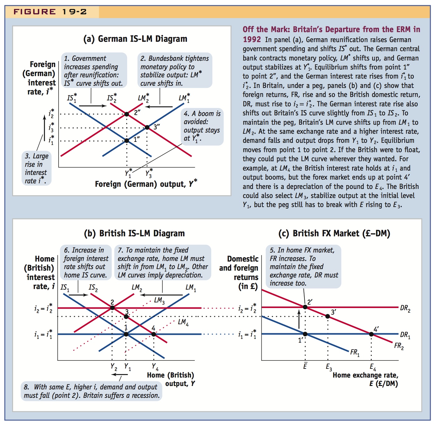
Panel (a) shows an IS-LM diagram for Germany, with German output on the horizontal axis and the German DM interest rate on the vertical axis. Panel (b) shows the British IS-LM diagram, with British output on the horizontal axis. Panel (c) shows the British forex market, with the exchange rate in pounds per mark. The vertical axes of panels (b) and (c) show returns in pounds, the home currency.
Initially, we suppose the three diagrams are in equilibrium as follows. In panel (a), at point 1″, German output is  and the DM interest rate
  . In panel (b), at point 1, British output is Y1 and the pound interest rate is i1. In panel (c), at point 1′, the pound is pegged to the DM at the fixed rate
  and expected depreciation is zero. The trilemma tells us that monetary policy autonomy is lost in Britain: the British interest rate must equal the German interest rate, so there is uncovered interest parity with
  .
.
A Shock in Germany With the scene set, our story begins with a threat to the ERM from an unexpected source. The countries of Eastern Europe began their transition away from Communism, a process that famously began with the fall of the Berlin Wall in 1989. After the wall fell, the reunification of East and West Germany was soon under way. Because the economically backward East Germany required significant funds to support social services, pay unemployment benefits, modernize infrastructure, and so on, the reunification imposed large fiscal costs on Germany, but West Germans were willing to pay these costs to see their country united. As we know from the previous chapter, an increase in German government consumption G* can be represented as a shift to the right in the German IS curve, from  to
to  in panel (a). This shift would have moved the German economy’s equilibrium from point 1″ to point 3″. All else equal, the model predicts an increase in German interest rates from to
  and a boom in German output from to
  2. This was indeed what started to happen.
The next chapter in the story involves the Bundesbank’s response to the German government’s expansionary fiscal policy. The Bundesbank was afraid that the boom in German output might cause an increase in German rates of inflation, and it wanted to avoid that outcome. Using its policy autonomy, the Bundesbank tightened its monetary policy by contracting the money supply and raising interest rates. This policy change is seen in the upward shift of the German LM curve, from  to
to  in panel (a). We suppose that the Bundesbank stabilizes German output at its initial level by raising German interest rates to the even higher level of
  .3
.3
309
310
Choices for the Other ERM Countries What happened in the countries of the ERM that were pegging to the DM? We examine what these events implied for Britain, but the other ERM members faced the same problems. The IS-LM-FX model tells us that events in Germany have two implications for the British IS-LM-FX model. First, as the German interest rate i* rises, the British foreign return curve FR shifts up in the British forex market (to recap: German deposits pay higher interest, all else equal). Second, as the German interest rate i* rises, the British IS curve shifts out (to recap: at any given British interest rate, the pound has to depreciate more, boosting British demand via expenditure switching). Now we only have to figure out how much the British IS curve shifts, what the British LM curve is up to, and hence how the equilibrium outcome depends on British policy choices.
Choice 1: Float and Prosper? First, let us suppose that in response to the increase in the German interest rate i*, the Bank of England had left British interest rates unchanged at i1 and suppose British fiscal policy had also been left unchanged. In addition, let’s assume that Britain would have allowed the pound-DM exchange rate to float in the short run. For simplicity we also assume that in the long run, the expected exchange rate remains unchanged, so that the long-run future expected exchange rate Ee remains unchanged at .
With these assumptions in place, let’s look at what happens to the investment component of demand: in Britain, I would be unchanged at I(i1). In the forex market in panel (c), the Bank of England, as assumed, holds the domestic return DR1 constant at i1. With the foreign return rising from FR1 to FR2 and the domestic return constant at DR1, the new equilibrium would be at 4′ and the British exchange rate rises temporarily to E4. Thus, if the Bank of England doesn’t act, the pound would have to depreciate to E4 against the DM; it would float, contrary to the ERM rules.
Now think about the effects of this depreciation on the trade balance component of demand: the British trade balance would rise because a nominal depreciation is also a real depreciation in the short run, given sticky prices.4 As we saw in the previous chapter, British demand would therefore increase, as would British equilibrium output.
To sum up the result after all these adjustments occur, an increase in the foreign interest rate always shifts out the home IS curve, all else equal as shown in panel (b): British interest rates would still be at i1, and British output would have risen to Y4, on the new IS curve IS2. To keep the interest rate at i1, as output rises, the Bank of England would have had to expand its money supply, shifting the British LM curve from LM1 to LM4, and causing the pound to depreciate to E4. If Britain were to float and depreciate the pound, it would experience a boom. But this would not have been compatible with Britain’s continued ERM membership.
Choice 2: Peg and Suffer? If Britain’s exchange rate were to stay pegged to the DM because of the ERM, however, the outcome for Britain would not be so rosy. In this scenario, the trilemma means that to maintain the peg, Britain would have to increase its interest rate and follow the lead of the center country, Germany. In panel (b), the pound interest rate would have to rise to the level  to maintain the peg. In panel (c), the domestic return would rise from DR1 to DR2 in step with the foreign return’s rise from FR1 to FR2, and the new FX market equilibrium would be at 2′. The Bank of England would accomplish this rise in DR by tightening its monetary policy and lowering the British money supply. In panel (b), under a peg, the new position of the IS curve at IS2 would imply an upward shift in the British LM curve, as shown by the move from LM1 to LM2. So the British IS-LM equilibrium would now be at point 2, with output at Y2. The adverse consequences for the British economy now become apparent. At point 2, as compared with the initial point 1, British demand has fallen. Why? British interest rates have risen (depressing investment demand I), but the exchange rate has remained at its pegged level (so there is no change in the trade balance). To sum up, what we have shown in this scenario is that the IS curve may have moved right a bit, but the opposing shift in the LM curve would have been even larger. If Britain were to stay pegged and keep its membership in the ERM, Britain would experience a recession.
311
In 1992 Britain found itself facing a decision between these two choices. As we have noted, if the British pound had been floating against the DM, then leaving interest rates unchanged would have been an option, and Britain could have achieved equilibrium at point 4 with a higher output, Y4. In fact, floating would have opened up the whole range of monetary policy options. For example, Britain could have chosen a mild monetary contraction by shifting the British LM curve from LM1 to LM3, moving equilibrium in panel (b) to point 3, stabilizing U.K. output at its initial level Y1, and allowing the FX market in panel (c) to settle at point 3′ with a mild depreciation of the exchange rate to E3.
What Happened Next? In September 1992, after an economic slowdown and after considerable last-minute dithering and turmoil, the British Conservative government finally decided that the benefits to Britain of being in ERM and the euro project were smaller than the costs suffered as a result of a German interest-rate hike in response to Germany-specific events. Two years after joining the ERM, Britain opted out.
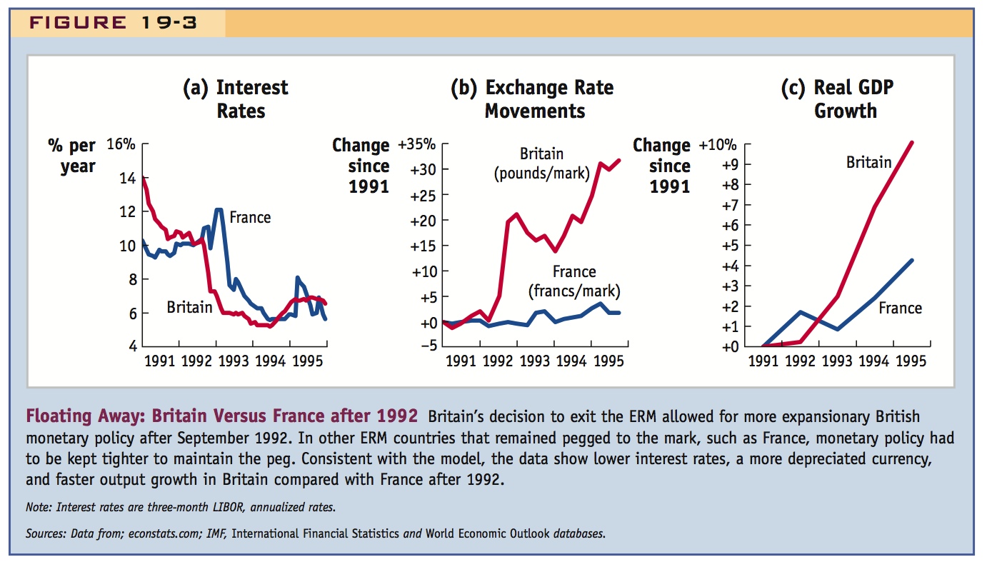
Did Britain make the right choice? In Figure 19-3, we compare the economic performance of Britain with that of France, a large European Union economy that maintained its ERM peg. After leaving the ERM in September 1992, Britain lowered interest rates [panel (a)] in the short run and depreciated its exchange rate against the DM [panel (b)]. In comparison, France never depreciated and had to maintain higher interest rates to keep the franc pegged to the DM until German monetary policy eased a year or two later. As our model would predict, the British economy boomed in subsequent years panel (c). The French suffered slower growth, a fate shared by most of the other countries that stayed in the ERM.
312
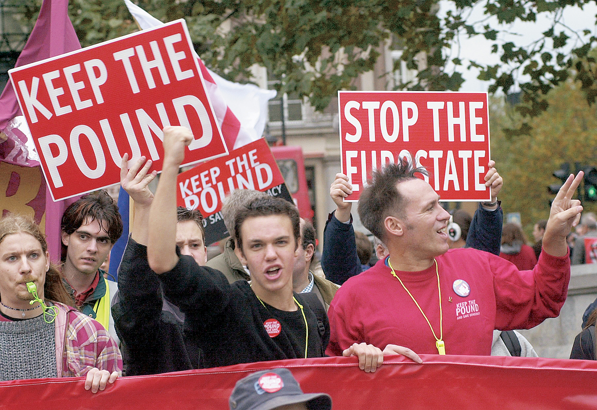
The British choice stands to this day. Although the option to rejoin the ERM has remained open since 1992, the idea of pegging to (much less joining) the euro is unpopular in Britain. All subsequent British governments have decided that the benefits of increased trade and economic integration with Europe were smaller than the associated costs of sacrificing British monetary autonomy.5
Work through both alternatives with the model. Point out that France found itself facing the same dilemma; the comparison between Britain and France will become explicit soon, so set the stage for here.
Compare and contrast Britain and France. England gave up the peg and prospered; France defended the peg, but suffered much slower growth. Go beyond this to mention that it lost reserves in maintaining the peg, creating speculative attacks. Say we will come back to this in the next chapter.
Key Factors in Exchange Rate Regime Choice: Integration and Similarity
We started this chapter with an application about the policy choice and tradeoffs Britain faced in 1992 when it needed to decide between a fixed exchange rate (peg) and a floating exchange rate (float).
At different times, British authorities could see the potential benefits of participating fully in an economically integrated single European market and the ERM fixed exchange rate system. The fixed exchange rate, for example, would lower the costs of economic transactions among the members of the ERM zone. But, especially in 1992, the British could also see that there would be times when the monetary policy being pursued by authorities in Germany would be out of line with policy that was best for Britain. The fundamental source of this divergence between what Britain wanted and what Germany wanted was that each country faced different shocks. The fiscal shock that Germany experienced after reunification was not felt in Britain or any other ERM country.
Now we talk about benefits as well as costs of fixed rates.
To better understand these trade-offs, and the decision to fix or float, we now examine the issues that are at the heart of this decision: economic integration as measured by trade and other transactions, and economic similarity, as measured by the similarity of shocks.
Economic Integration and the Gains in Efficiency
The term economic integration refers to the growth of market linkages in goods, capital, and labor markets among regions and countries. By lowering transaction costs, a fixed exchange rate might promote integration and increase economic efficiency.
313
Trade is the clearest example of an activity that volatile exchange rates might discourage. Stable exchange rates and prices encourage arbitrage and lower the costs of trade. But trade is not the only type of international economic activity likely to be discouraged by exchange rate fluctuations. Currency-related transaction costs and uncertainty also act as barriers to cross-border capital and labor flows.
Benefits
- The lesson: the greater the degree of economic integration between markets in the home country and the base country, the greater will be the volume of transactions between the two, and the greater will be the benefits the home country gains from fixing its exchange rate with the base country. As integration rises, the efficiency benefits of having a fixed exchange rate increase.
Economic Similarity and the Costs of Asymmetric Shocks
A fixed exchange rate can lead to costs when one country experiences a country-specific shock or asymmetric shock that is not shared by the other country.
The application on Britain and Germany showed why an asymmetric shock causes problems: it leads to a conflict between the policy goals of the two countries. In our example, German policy makers wanted to tighten monetary policy to offset a boom caused by a positive demand shock due to their expansionary fiscal policy. British policy makers did not want to implement the same policy: because they had not experienced the same shock, following the German monetary policy would have caused a recession in Britain.
Similar or symmetric shocks do not cause such problems. Imagine that Germany and Britain experience an identical expansionary demand shock. In this case, German and British monetary authorities would respond identically, raising interest rates by the same amount to stabilize output. This desired symmetric increase in interest rates does not conflict with Britain’s fixed exchange rate commitment. If interest rates were initially set at a common level, , they would be raised to a new higher level, . By raising its rates, Britain could stabilize output and stay pegged because uncovered interest parity is still satisfied. The exchange rate does not change, and even though Britain is pegging unilaterally to Germany, Britain has the interest rate it would choose even if it were floating and could make an independent monetary policy choice.
When a Home country unilaterally pegs to a Foreign country, asymmetric shocks impose costs on the home country in terms of lost output. When asymmetric shocks hit, the monetary policies that are best for Foreign and for Home will differ, and the peg means that Foreign’s policy choice will automatically be imposed on Home. In contrast, symmetric shocks do not impose any costs because the monetary policies that Foreign and Home want to pursue will be the same, and Foreign’s imposed choice will suit Home perfectly.
Real-world situations are more complex. Countries are not identical and shocks may be a mix of large and small, symmetric and asymmetric shocks.
Costs
- The lesson: if there is a greater degree of economic similarity between the home country and the base country (that is, if they face more symmetric shocks and fewer asymmetric shocks), then the economic stabilization costs to home of fixing its exchange rate to the base are smaller. As economic similarity rises, the stability costs of having a fixed exchange rate decrease.
314
Simple Criteria for a Fixed Exchange Rate
We can now set out a theory of exchange rate regime choice by considering the net benefits (benefits minus the costs) of pegging versus floating. Our discussions about integration and similarity have shown the following:
- As integration rises, the efficiency benefits of a fixed exchange rate increase.
- As symmetry rises, the stability costs of a fixed exchange rate decrease.
Our theory says that if market integration or symmetry increases, the net benefits of a fixed exchange rate also increase. If the net benefits are negative, the home country should float if the decision is based solely on its economic interests. If the net benefits are positive, the home country should fix.
This diagram summarizes the argument nicely. Make sure they understand the FX frontier and consider each of the numbered combinations. You will already have students asking where Europe fits in the diagram, or even the U.S.
Figure 19-4 illustrates the theory in a symmetry-integration diagram in which the horizontal axis measures the degree of economic integration between a pair of locations, say, A and B, and the vertical axis measures the symmetry of the shocks experienced by the pair A and B.
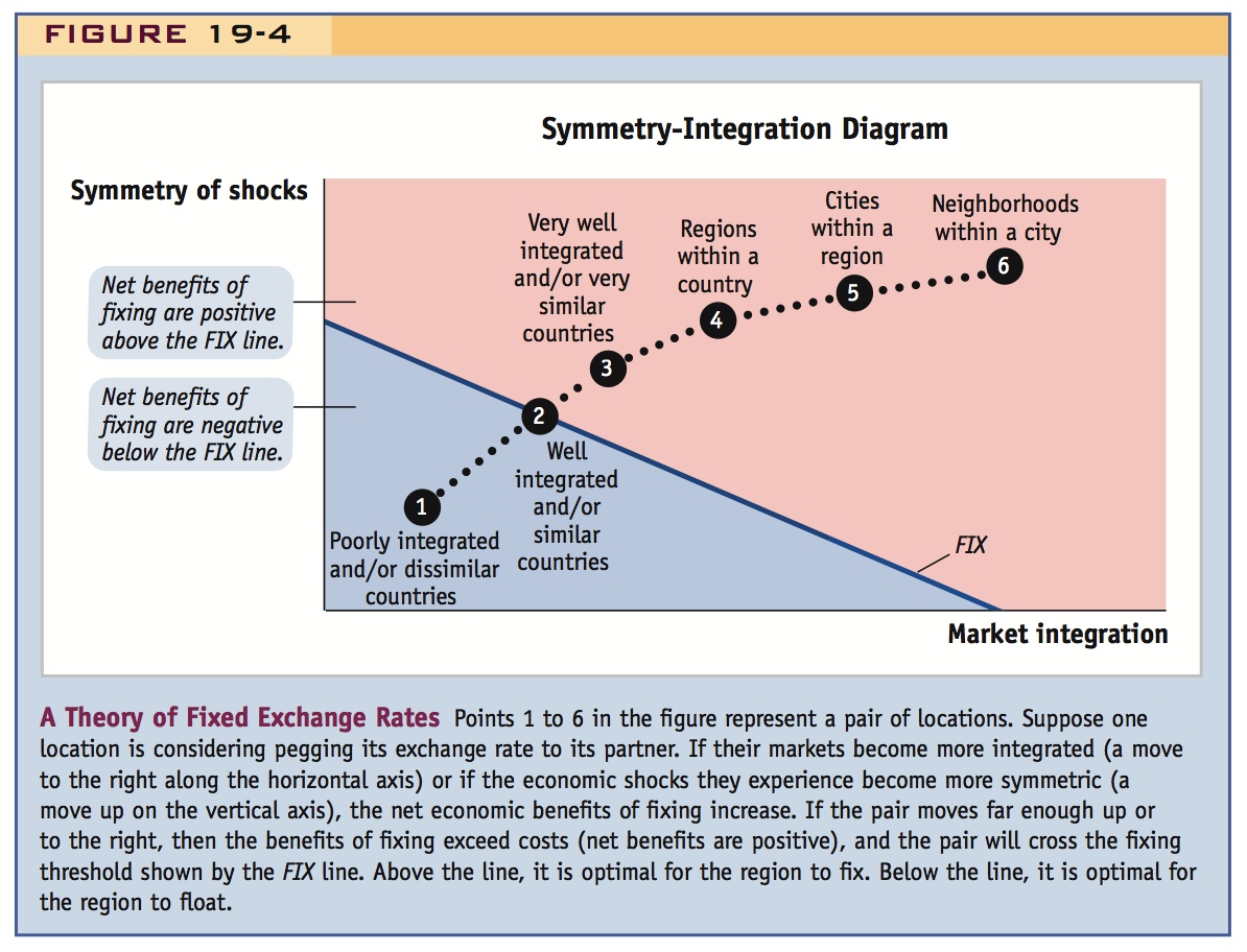
We use the figure to see whether A should peg unilaterally to B (or vice versa). Suppose conditions change and the pair moves up and to the right, for example, from point 1 toward point 6. Along this path, integration and symmetry are both increasing, so the net benefits of fixing are also increasing. At some critical point (point 2 in the graph), the net benefits turn positive. Before that point, floating is best. After that point, fixing is best.
315
Our argument is more general: whatever the direction of the path, as long as it moves up and to the right, it must cross some threshold like point 2 beyond which benefits outweigh costs. Thus, there will exist a set of points—a downward-sloping line passing through point 2—that delineates this threshold. We refer to this threshold as the FIX line. Points above the FIX line satisfy the economic criteria for a fixed exchange rate.
What might different points on this chart mean? If we are at point 6, we might think of A and B as neighborhoods in a city—they are very well integrated and an economic shock is usually felt by all neighborhoods in the city. If A and B were at point 5, they might be two cities. If A and B were at point 4, they might be the regions of a country, and still above the FIX line. If A and B were at point 3, they might be neighboring, well-integrated countries with few asymmetric shocks. Point 2 is right on the borderline. If A and B were at point 1, they might be less well-integrated countries with more asymmetric shocks and our theory says they should float.
The key prediction of our theory is this: pairs of countries above the FIX line (more integrated, more similar shocks) will gain economically from adopting a fixed exchange rate. Those below the FIX line (less integrated, less similar shocks) will not.
In a moment, we develop and apply this theory further. But first, let’s see if there is evidence to support the theory’s two main assumptions: Do fixed exchange rates deliver trade gains through integration? Do they impose stability costs by limiting monetary policy options?
a. Benefits Measured by Trade Levels
Trade expanded rapidly during the gold standard. Shambaugh and Klein provide evidence that direct pegs (between two countries) promote trade.
b. Benefits Measured by Price Convergence
Empirical research suggests that exchange rate volatility reduces the speed of convergence of the prices of baskets of goods and is associated with larger deviations from LOOP for individual goods.
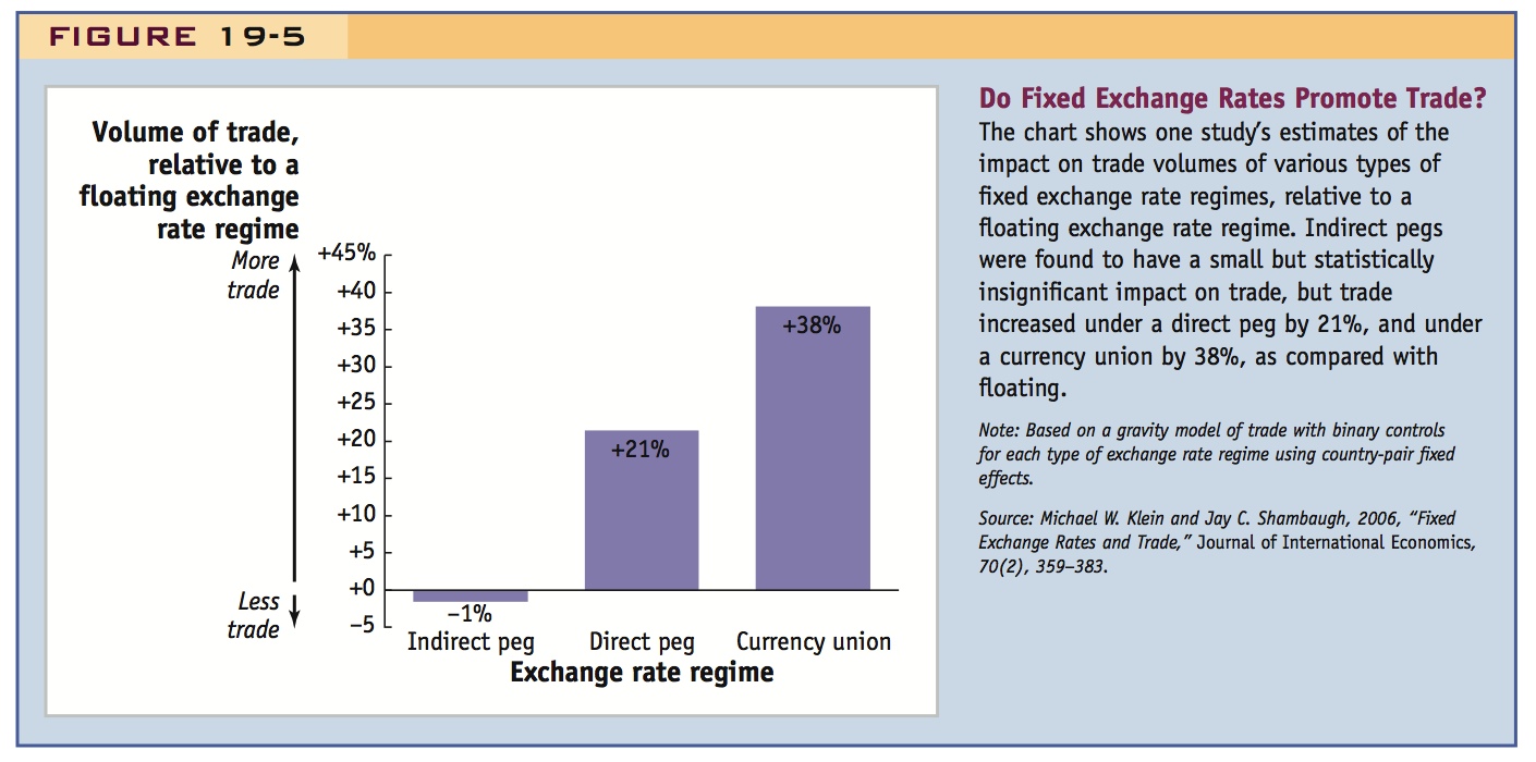
Do Fixed Exchange Rates Promote Trade?
The single most powerful argument for a fixed exchange rate is that it may boost trade by eliminating trade-hindering costs. The idea is an old one. In 1878, the United States had yet to re-adopt the gold standard following the Civil War. Policy makers were debating whether going back on gold made sense, and J. S. Moore, a U.S. Treasury official testifying before Congress, was questioned on the subject:
Question: Do you not think that the use of a common standard of value has a tendency to promote a free commercial interchange between the various countries using it?
Answer: If two countries, be they ever so distant from each other, should have the same standard of money…there would be no greater harmonizer than such an exchange.
Benefits Measured by Trade Levels As we have noted, this was the conventional wisdom among policy makers in the late nineteenth and early twentieth centuries, and research by economic historians has found strong support for their views: all else equal, two countries adopting the gold standard had bilateral trade levels 30% to 100% higher than comparable pairs of countries that were off the gold standard.6 Thus, it appears that the gold standard did promote trade.
316
What about fixed exchange rates today? Do they promote trade? Economists have exhaustively tested this hypothesis using increasingly sophisticated statistical methods. We can look at some evidence from a recent study in which country pairs A–B were classified in four different ways:
- The two countries are using a common currency (i.e., A and B are in a currency union or A has unilaterally adopted B’s currency).
- The two countries are linked by a direct exchange rate peg (i.e., A’s currency is pegged to B’s).
- The two countries are linked by an indirect exchange rate peg, via a third currency (i.e., A and B have currencies pegged to C but not directly to each other).
- The two countries are not linked by any type of peg (i.e., their currencies float against each other, even if one or both might be pegged to some other third currency).
Using this classification and trade data from 1973 to 1999, economists Jay Shambaugh and Michael Klein compared bilateral trade volumes for all pairs under the three pegged regimes (a) through (c) with the benchmark level of trade under a floating regime (d) to see if there were any systematic differences. They also used careful statistical techniques to control for other factors and to address possible reverse causality (that is, to eliminate the possibility that higher trade might have caused countries to fix their exchange rates). Figure 19-5 shows their key estimates, according to which currency unions increased bilateral trade by 38% relative to floating regimes. They also found that the adoption of a fixed exchange rate would promote trade, but only for the case of direct pegs. Adopting a direct peg increased bilateral trade by 21% compared with a floating exchange rate. Indirect pegs had a negligible and statistically insignificant effect.7
317
Benefits Measured by Price Convergence The effect of exchange rate regimes on trade levels is one way to evaluate the impact of currency arrangements on international market integration, and it has been extensively researched. Another body of research examines the relationship between exchange rate regimes and price convergence. These studies use the law of one price (LOOP) and purchasing power parity (PPP) as criteria for measuring market integration. If fixed exchange rates promote trade by lowering transaction costs, then differences between prices (measured in a common currency) should be smaller among countries with pegged rates than among countries with floating rates. In other words, LOOP and PPP should be more likely to hold under a fixed exchange rate than under a floating regime. (Recall that price convergence underlies the gains-from-trade argument.)
Statistical methods can be used to detect how large price differences must be between two locations before arbitrage begins. Research on prices of baskets of goods shows that as exchange rate volatility increases (as it does when currencies float), price differences widen, and the speed at which prices in the two markets converge decreases. These findings offer support for the hypothesis that fixed exchange rates promote arbitrage and price convergence.8
Economists have also studied convergence in the prices of individual goods. For example, several studies focused on Europe have looked at the prices of various goods in different countries (e.g., retail prices of cars and TV sets, and the prices of Marlboro cigarettes in duty-free shops). These studies showed that higher exchange rate volatility is associated with larger price differences between locations. In particular, while price gaps still remain for many goods, the “in” countries (members of the ERM and now the Eurozone) saw prices converge much more than the “out” countries.9
A compelling result to discuss: The answer is yes, significantly.
Conclusion: The answer is yes here, too.
a. The Trilemma, Policy Constraints, and Interest Rate Correlations
Empirical evidence suggests that fixed rates with capital mobility permit little monetary autonomy.
b. Costs of Fixing Measured by Output Volatility
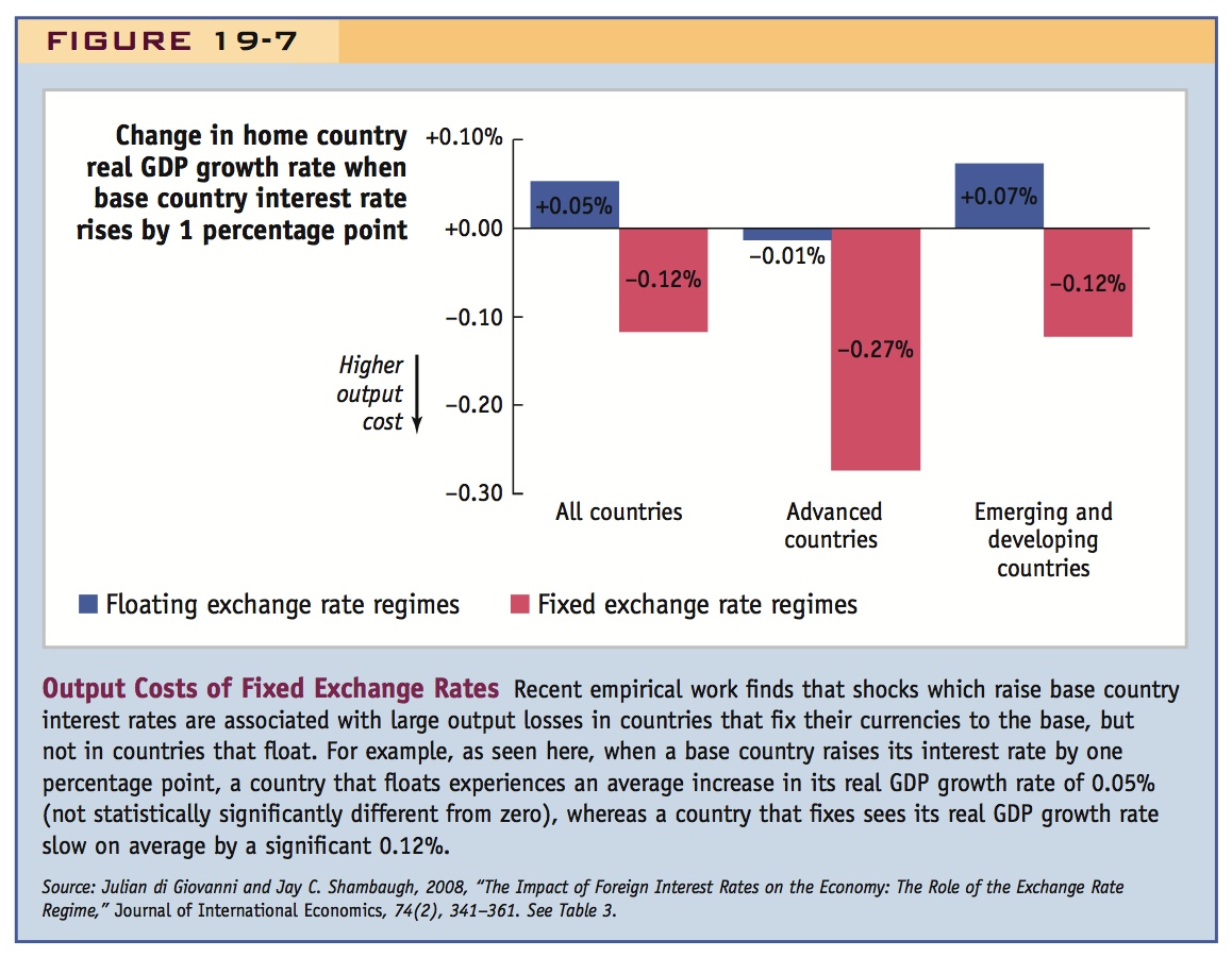
Under fixed rates, an increase in base country interest rates should reduce domestic income. Giovanni and Shambaugh show that this tends to occur under fixed rates, but not under flexible rates.
Do Fixed Exchange Rates Diminish Monetary Autonomy and Stability?
Probably the single most powerful argument against a fixed exchange rate is provided by the trilemma. An economy that unilaterally pegs to a foreign currency sacrifices its monetary policy autonomy.
We have seen the result many times now. If capital markets are open, arbitrage in the forex market implies uncovered interest parity. If the exchange rate is fixed, expected depreciation is zero, and the home interest rate must equal the foreign interest rate. The stark implication is that when a country pegs, it relinquishes its independent monetary policy: it has to adjust the money supply M at all times to ensure that the home interest rate i equals the foreign interest rate i* (plus any risk premium).
318
The preceding case study of Britain and the ERM is one more example: Britain wanted to decouple the British interest rate from the German interest rate. To do so, it had to stop pegging the pound to the German mark. Once it had done that, instead of having to contract the British economy as a result of unrelated events in Germany, it could maintain whatever interest rate it thought was best suited to British economic interests.
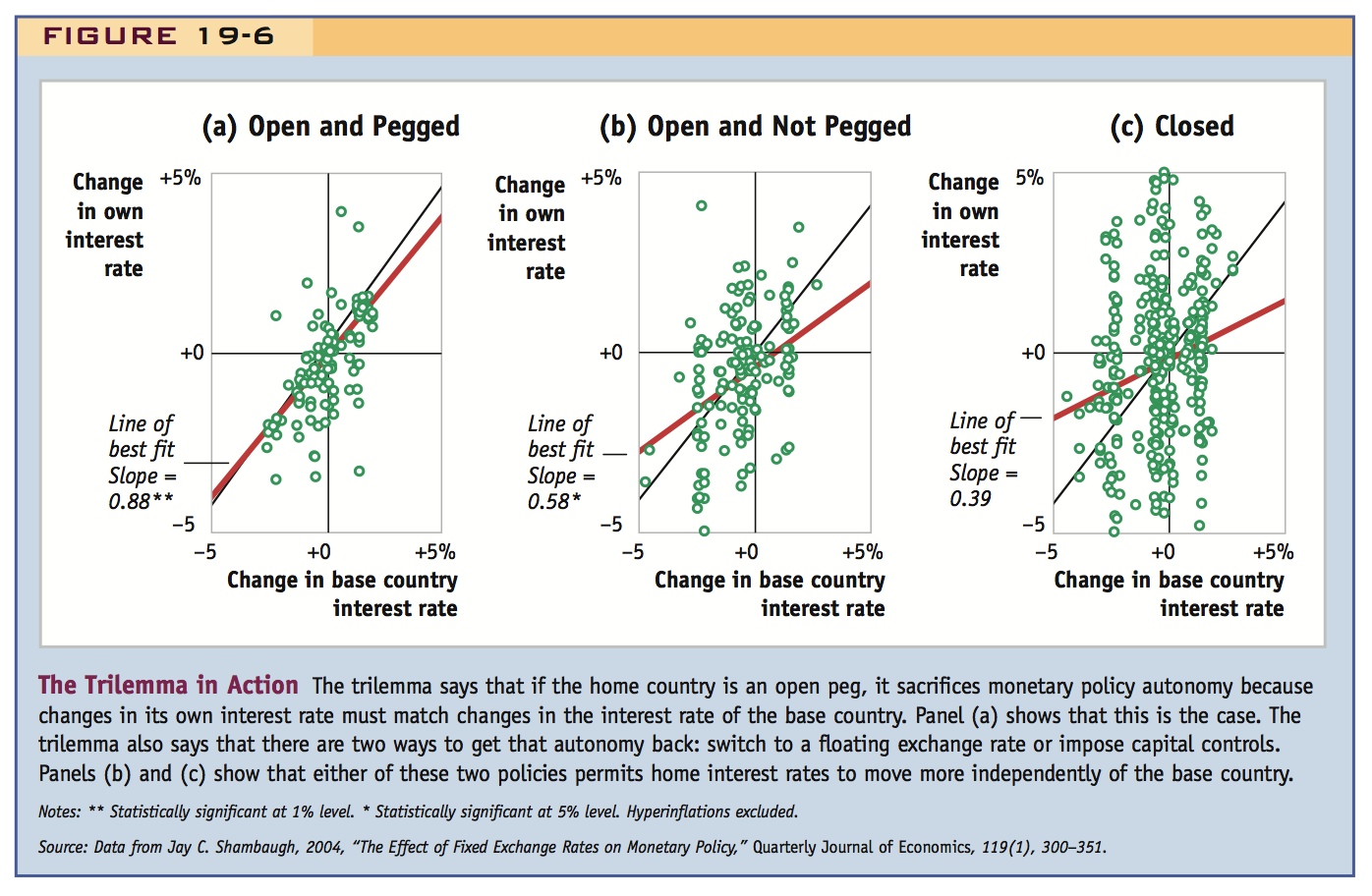
The Trilemma, Policy Constraints, and Interest Rate Correlations Is the trilemma truly a binding constraint? Economist Jay Shambaugh tested this proposition, and Figure 19-6 shows some evidence using his data. As we have seen, there are three main solutions to the trilemma. A country can do the following:
- Opt for open capital markets, with fixed exchange rates (an “open peg”).
- Opt to open its capital market but allow the currency to float (an “open nonpeg”).
- Opt to close its capital markets (“closed”).
In case 1, changes in the country’s interest rate should match changes in the interest rate of the base country to which it is pegging. In cases 2 and 3, there is no need for the country’s interest rate to move in step with the base.
319
Figure 19-6 displays evidence for the trilemma. On the vertical axis is the annual change in the domestic interest rate; on the horizontal axis is the annual change in the base country interest rate. The trilemma says that in an open peg the two changes should be same and the points should lie on the 45-degree line. Indeed, for open pegs, shown in panel (a), the correlation of domestic and base interest rates is high and the line of best fit has a slope very close to 1. There are some deviations (possibly due to some pegs being more like bands), but these findings show that open pegs have very little monetary policy autonomy. In contrast, for the open nonpegs, shown in panel (b), and closed economies, shown in panel (c), domestic interest rates do not move as much in line with the base interest rate, the correlation is weak, and the slopes are much smaller than 1. These two regimes allow for some monetary policy autonomy.10
Costs of Fixing Measured by Output Volatility The preceding evidence suggests that nations with open pegs have less monetary independence. But it does not tell us directly whether they suffer from greater output instability because their monetary authorities cannot use monetary policy to stabilize output when shocks hit. Some studies have found that, on average, the volatility of output growth is much higher under fixed regimes.11 However, a problem in such studies is that countries often differ in all kinds of characteristics that may affect output volatility, not just the exchange rate regime—and the results can be sensitive to how one controls for all these other factors.12
In the search for cleaner evidence, some recent research has focused on a key prediction of the IS-LM-FX model: all else equal, an increase in the base-country interest rate should cause output to fall in a country that fixes its exchange rate to the base country. This decline in output occurs because countries that fix have to tighten their monetary policy and raise their interest rate to match that of the base country. In contrast, countries that float do not have to follow the base country’s rate increase and can use their monetary policy autonomy to stabilize output, by lowering their interest rate and/or allowing their currency to depreciate. Economists Julian di Giovanni and Jay Shambaugh looked at changes in base-country interest rates (say, the U.S. dollar or euro rates) and examined the correlation of these base interest rate changes with changes in GDP in a large sample of fixed and floating nonbase countries. The results, shown in Figure 19-7, confirm the theory’s predictions: when a base country increases its interest rate, it spreads economic pain to those countries pegging to it, but not to the countries that float. These findings confirm that one cost of a fixed exchange rate regime is a more volatile level of output.
These are also compelling. Put these on the screen and ask the students to figure out what these imply.
Here too, ask students to interpret this.
320