2 Ricardian Model
1. Objectives:
Formal development of the Ricardian model; demonstration that a country should export the good for which it has a comparative advantage
2. The Home Country
a. Assumptions:
Two goods, wheat and cloth; one factor, labor, supplied inelastically and mobile across sectors; constant marginal products, MPLc, MPLw.
b. Home Production Possibilities Frontier (PPF)
Derivation; slope of PPF equals the negative of the ratio of the marginal products, MPLc/MPLw interpretation of slope of the PPF as opportunity cost of wheat.
c. Home Indifference Curve
Same as the indifference curves of individual consumers encountered in micro classes, except that they represent preferences of the whole country.
d. Home Equilibrium (Autarky)
Tangency of PPF and indifference curve.
e. Opportunity Cost and Prices
In autarky, prices of goods will reflect their opportunity costs of production.
f. Wages
In autarky, PW/PC = MPLC/MPLW: Without trade the relative price of wheat must equal its opportunity cost.
3. The Foreign Country
Foreign is less productive in both sectors, so it has an absolute disadvantage.
a. Foreign PPF
Derive foreign PPF; foreign autarky relative price = foreign opportunity cost.
b. Comparative Advantage
i. Home economy is more productive in both sectors. However, it has a comparative advantage in wheat. Therefore the relative price of wheat is lower at home than abroad when there is no trade.
ii. Foreign has a comparative advantage in cloth. Therefore the relative price of cloth is lower abroad than at home when there is no trade.
iii. Foreign should export cloth to the home country, even though it is at an absolute disadvantage in both goods.
In developing the Ricardian model of trade, we will work with an example similar to that used by Ricardo; instead of wine and cloth, however, the two goods will be wheat and cloth. Wheat and other grains (including barley, rice, and so on) are major exports of the United States and Europe, while many types of cloth are imported into these countries. In our example, the home country (we will call it just “Home”) will end up with this trade pattern, exporting wheat and importing cloth.
The Home Country
This may require some elaboration:
1. Write down the actual production function and draw a picture of it. Compare it to the usual picture with diminishing returns that students are familiar with from their micro classes.
2. Emphasize that this is only a useful simplification, and that adding diminishing returns wouldn't change much in this setting.
3. However, some students will recognize this as a Leontief technology, so provide an alternative interpretation of the MPLs as unit labor coefficients.
To simplify our example, we will ignore the role of land and capital and suppose that both goods are produced with labor alone. In Home, one worker can produce 4 bushels of wheat or 2 yards of cloth. This production can be expressed in terms of the marginal product of labor (MPL) for each good. Recall from your study of microeconomics that the marginal product of labor is the extra output obtained by using one more unit of labor.2 In Home, one worker produces 4 bushels of wheat, so MPLW = 4. Alternatively, one worker can produce 2 yards of cloth, so MPLC = 2.

To reinforce this intuitive argument, derive the PPF algebraically: Start with the labor constraint, then substitute in the production functions.
Let the students create their own numerical examples, picking a labor endowment and MPLs and then deriving the PPF.
Home Production Possibilities Frontier Using the marginal products for producing wheat and cloth, we can graph Home’s production possibilities frontier (PPF). Suppose there are  = 25 workers in the home country (the bar over the letter L indicates our assumption that the amount of labor in Home stays constant). If all these workers were employed in wheat, they could produce QW = MPLW · = 4 · 25 = 100 bushels. Alternatively, if they were all employed in cloth, they could produce QC = MPLC · = 2 · 25 = 50 yards. The production possibilities frontier is a straight line between these two points at the corners, as shown in Figure 2-1. The straight-line PPF, a special feature of the Ricardian model, follows from the assumption that the marginal products of labor are constant. That is, regardless of how much wheat or cloth is already being produced, one extra hour of labor yields an additional 4 bushels of wheat or 2 yards of cloth. There are no diminishing returns in the Ricardian model because it ignores the role of land and capital.
Briefly depict what the PPF would look like if there were diminishing returns. They are often habituated to a concave PPF.
34
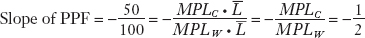
Given this property, the slope of the PPF in Figure 2-1 can be calculated as the ratio of the quantity of cloth produced to the quantity of wheat produced at the corners, as follows:
To set the stage for explaining the gains from trade it helps to actually refer to the opportunity cost of wheat as the MARGINAL COST of wheat in terms of cloth. The idea that more of a good should be produced if P > MC will ring bells.
Ignoring the minus sign, the slope equals the ratio of marginal products of the two goods. The slope is also the opportunity cost of wheat, the amount of cloth that must be given up to obtain one more unit of wheat.3 To see this, suppose that QW is increased by 1 bushel. It takes one worker to produce 4 bushels of wheat, so increasing QW by 1 bushel means that one-quarter of a worker’s time must be withdrawn from the cloth industry and shifted into wheat production. This shift would reduce cloth output by  yard, the amount of cloth that could have been produced by one-quarter of a worker’s time. Thus, yard of cloth is the opportunity cost of obtaining 1 more bushel of wheat and is the slope of the PPF.
2 A special assumption of the Ricardian model is that there are no diminishing returns to labor, so the marginal product of labor is constant. That assumption will no longer be made in the next chapter, when we introduce capital and land, along with labor, as factors of production.
Beware! Students may not be as familiar with basic consumer theory as you may think. You may have to digress to review some of these tools.
Home Indifference Curve With this production possibilities frontier, what combination of wheat and cloth will Home actually produce? The answer depends on the country’s demand for each of the two goods. There are several ways to represent demand in the Home economy, but we will start by using indifference curves. Each indifference curve shows the combinations of two goods, such as wheat and cloth, that a person or economy can consume and be equally satisfied.
35
In Figure 2-2, the consumer is indifferent between points A and B, for example. Both of these points lie on an indifference curve U1 associated with a given level of satisfaction, or utility. Point C lies on a higher indifference curve U2, indicating that it gives a higher level of utility, whereas point D lies on a lower indifference curve U0, indicating that it gives a lower level of utility. It is common to use indifference curves to reflect the utility that an individual consumer receives from various consumption points. In Figure 2-2, we go a step further, however, and apply this idea to an entire country. That is, the indifference curves in Figure 2-2 show the preferences of an entire country. The combinations of wheat and cloth on U0 give consumers in the country lower utility than the combinations on indifference curve U1, which in turn gives lower utility than the combinations of wheat and cloth on U2.

Home Equilibrium In the absence of international trade, the production possibilities frontier acts like a budget constraint for the country, and with perfectly competitive markets, the economy will produce at the point of highest utility subject to the limits imposed by its PPF. The point of highest utility is at point A in Figure 2-2, where Home consumes 25 yards of cloth and 50 bushels of wheat. This bundle of goods gives Home the highest level of utility possible (indifference curve U1) given the limits of its PPF. Notice that Home could produce at other points such as point D, but this point would give a lower level of utility than point A (i.e., point D would offer lower utility because U0 is lower than U1). Other consumption points, such as C, would give higher levels of utility than point A but cannot be obtained in the absence of international trade because they lie outside of Home’s PPF.
36
We will refer to point A as the “no-trade” or the “pre-trade” equilibrium for Home.4 What we really mean by this phrase is “no international trade.” The Home country is able to reach point A by having its own firms produce wheat and cloth and sell these goods to its own consumers. We are assuming that there are many firms in each of the wheat and cloth industries, so the firms act under perfect competition and take the market prices for wheat and cloth as given. The idea that perfectly competitive markets lead to the highest level of well-being for consumers—as illustrated by the highest level of utility at point A—is an example of the “invisible hand” that Adam Smith (1723–1790) wrote about in his famous book The Wealth of Nations. Like an invisible hand, competitive markets lead firms to produce the amount of goods that results in the highest level of well-being for consumers.
4 We also refer to point A as the “autarky equilibrium,” because “autarky” means a situation in which the country does not engage in international trade.
Opportunity Cost and Prices Whereas the slope of the PPF reflects the opportunity cost of producing one more bushel of wheat, under perfect competition the opportunity cost of wheat should also equal the relative price of wheat, as follows from the economic principle that price reflects the opportunity cost of a good. We can now check that this equality between the opportunity cost and the relative price of wheat holds at point A.
Wages We solve for the prices of wheat and cloth using an indirect approach, by first reviewing how wages are determined. In competitive labor markets, firms hire workers up to the point at which the cost of one more hour of labor (the wage) equals the value of one more hour of production. In turn, the value of one more hour of labor equals the amount of goods produced in that hour (the marginal product of labor) times the price of the good (PW for the price of wheat and PC for the price of cloth). That is to say, in the wheat industry, labor will be hired up to the point at which the wage equals PW · MPLW, and in the cloth industry labor will be hired up to the point at which the wage equals PC · MPLC.
Students often find perfect factor mobility implausible. Explain that this is implicitly a long-run story. Also explain that sectoral shifts in labor occur more quickly in some countries rather than in others, e.g. perhaps the U.S. versus Europe.
If we assume that labor is perfectly free to move between these two industries and that workers will choose to work in the industry for which the wage is highest, then wages must be equalized across the two industries. If the wages were not the same in the two industries, laborers in the low-wage industry would have an incentive to move to the high-wage industry; this would, in turn, lead to an abundance of workers and a decrease in the wage in the high-wage industry and a scarcity of workers and an increase in the wage in the low-wage industry. This movement of labor would continue until wages are equalized between the two industries.
We can use the equality of the wage across industries to obtain the following equation:
PW · MPLW = PC · MPLC
Encourage students to keep units of measurement straight, so that both sides of this equation are measured in yards of cloth per bushel of wheat.
By rearranging terms, we see that
PW/PC = MPLC/MPLW
37
If you've called the opportunity cost of wheat the marginal cost of wheat (see above), then you can explain that in the autarky equilibrium P = MC, which connects with some students.
The right-hand side of this equation is the slope of the production possibilities frontier (the opportunity cost of obtaining one more bushel of wheat) and the left-hand side of the equation is the relative price of wheat, as we will explain in the next paragraph. This equation says that the relative price of wheat (on the left) and opportunity cost of wheat (on the right) must be equal in the no-trade equilibrium at point A.
To understand why we measure the relative price of wheat as the ratio PW/PC, suppose that a bushel of wheat costs $3 and a yard of cloth costs $6. Then $3/$6 = , which shows that the relative price of wheat is , that is, of a yard of cloth (or half of $6) must be given up to obtain 1 bushel of wheat (the price of which is $3). A price ratio like PW/PC always denotes the relative price of the good in the numerator (wheat, in this case), measured in terms of how much of the good in the denominator (cloth) must be given up. In Figure 2-2, the slope of the PPF equals the relative price of wheat, the good on the horizontal axis.
The Foreign Country
Now let’s introduce another country, Foreign, into the model. We will assume that Foreign’s technology is inferior to Home’s so that it has an absolute disadvantage in producing both wheat and cloth as compared with Home. Nevertheless, once we introduce international trade, we will still find that Foreign will trade with Home.
Foreign Production Possibilities Frontier Suppose that one Foreign worker can produce 1 bushel of wheat ( = 1), or 1 yard of cloth (
 = 1), whereas recall that a Home worker can produce 4 bushels of wheat or 2 yards of cloth. Suppose that there are
  = 100 workers available in the Foreign country. If all these workers were employed in wheat, they could produce · = 100 bushels, and if they were all employed in cloth, they could produce · = 100 yards. Foreign’s production possibilities frontier (PPF) is thus a straight line between these two points, with a slope of −1, as shown in Figure 2-3.

Construct an example where the foreign PPF is entirely inside the domestic PPF. This will provide a particularly compelling case of why trade based upon comparative advantage is beneficial.
You might find it helpful to think of the Home country in our example as the United States or Europe and the Foreign country as the “rest of the world.” Empirical evidence supports the idea that the United States and Europe have the leading technologies in many goods and an absolute advantage in the production of both wheat and cloth. Nevertheless, they import much of their clothing and textiles from abroad, especially from Asia and Latin America. Why does the United States or Europe import these goods from abroad when they have superior technology at home? To answer this question, we want to focus on the comparative advantage of Home and Foreign in producing the two goods.
Comparative Advantage In Foreign, it takes one worker to produce 1 bushel of wheat or 1 yard of cloth. Therefore, the opportunity cost of producing 1 yard of cloth is 1 bushel of wheat. In Home, one worker produces 2 yards of cloth or 4 bushels of wheat. Therefore, Home’s opportunity cost of a bushel of wheat is a yard of cloth, and its opportunity cost of a yard of cloth is 2 bushels of wheat. Based on this comparison, Foreign has a comparative advantage in producing cloth because its opportunity cost of cloth (which is 1 bushel of wheat) is lower than Home’s opportunity cost of cloth (which is 2 bushels of wheat). Conversely, Home has a comparative advantage in producing wheat because Home’s opportunity cost of wheat (which is yard of cloth) is lower than Foreign’s (1 yard of cloth). In general, a country has a comparative advantage in a good when it has a lower opportunity cost of producing it than does the other country. Notice that Foreign has a comparative advantage in cloth even though it has an absolute disadvantage in both goods.
38
As before, we can represent Foreign’s preferences for wheat and cloth with indifference curves like those shown in Figure 2-4. With competitive markets, the economy will produce at the point of highest utility for the country, point A*, which is the no-trade equilibrium in Foreign. The slope of the PPF, which equals the opportunity cost of wheat, also equals the relative price of wheat.5 Therefore, in Figure 2-4, Foreign’s no-trade relative price of wheat is  = 1. Notice that this relative price exceeds Home’s no-trade relative price of wheat, which is PW/PC = . This difference in these relative prices reflects the comparative advantage that Home has in the production of wheat.6
5 Remember that the slope of the PPF (ignoring the minus sign) equals the relative price of the good on the horizontal axis—wheat in Figure 2-4. Foreign has a steeper PPF than Home as shown in Figure 2-2, so Foreign’s relative price of wheat is higher than Home’s. The inverse of the relative price of wheat is the relative price of cloth, which is lower in Foreign.
6 Taking the reciprocal of the relative price of wheat in each country, we also see that Foreign’s no-trade relative price of cloth is = 1, which is less than Home’s no-trade relative price of cloth, PC/PW = 2. Therefore, Foreign has a comparative advantage in cloth.

Another example: productivity differentials between the U.S. and Mexico.
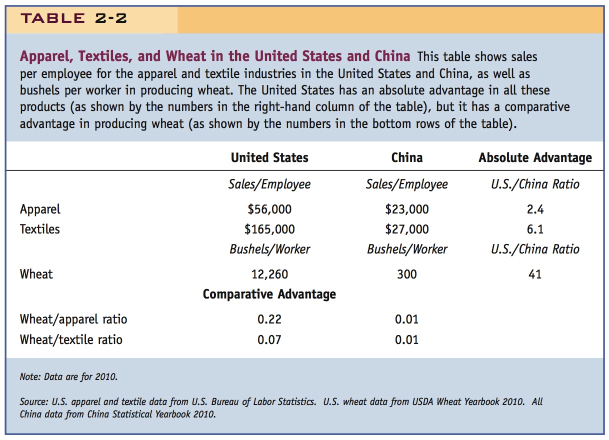
The U.S. has an absolute advantage over China, but has a comparative advantage in wheat. So the U.S. exports wheat to China in exchange for apparel and textiles.
Comparative Advantage in Apparel, Textiles, and Wheat
The U.S. textile and apparel industries face intense import competition, especially from Asia and Latin America. Employment in this industry in the United States fell by more than 80%, from about 1.7 million people in 1990 to about 300,000 in 2011. An example of this import competition can be seen in one U.S. fabric manufacturer, Burlington Industries, which announced in January 1999 that it would reduce its production capacity by 25% because of increased imports from Asia. Burlington closed seven plants and laid off 2,900 people, approximately 17% of its domestic force. After the layoffs, Burlington Industries employed 17,400 people in the United States. Despite these reductions in employment, textiles and apparel remains an important industry in some cities: Los Angeles had about 2,500 business establishments in the apparel industry in 2010, and New York had about 800.7
39
The average sales per employee for all U.S. apparel producers was $56,000 in 2010, as shown in Table 2-2. The textile industry, producing the fabric and material inputs for apparel, is even more productive, with annual sales per employee of $165,000 in the United States. In comparison, the average employee in China produces $23,000 of sales per year in the apparel industry and $27,000 in the textile industry. Thus, an employee in the United States produces $56,000/$23,000 = 2.4 times more apparel sales than an employee in China and $165,000/$27,000 = 6.1 times more textile sales. This ratio is shown in Table 2-2 in the column labeled “Absolute Advantage.” It illustrates how much more productive U.S. labor is in these industries relative to Chinese labor. The United States clearly has an absolute advantage in both these industries, so why does it import so much of its textiles and apparel from Asia, including China?
40
The answer can be seen by also comparing the productivities in the wheat industry. The typical wheat farm in the United States grows more than 12,000 bushels of wheat per worker (by which we mean either the farmer or an employee). In comparison, the typical wheat farm in China produces only 300 bushels of wheat per worker, so the U.S. farm is 12,260/300 = 41 times more productive! The United States clearly has an absolute advantage in the textile and apparel and wheat industries.
But China has the comparative advantage in both apparel and textiles, as illustrated by the rows labeled “Comparative Advantage.” Dividing the marginal product of labor in wheat by the marginal product of labor in apparel give us the opportunity cost of apparel. In the United States, for example, this ratio is 12,260/$56,000 = 0.22 bushels/$, indicating that 0.22 bushels of wheat must be foregone to obtain an extra dollar of sales in apparel. In textiles, the U.S. ratio is 12,260/$165,000 = 0.07 bushels/$, so that 0.07 bushels of wheat must be foregone to obtain an extra dollar in textile sales. These ratios are much smaller in China: only 300/$23,000 or 300/$27,000 ∼ 0.01 bushels of wheat must be foregone to obtain $1 of extra sales in either textiles or apparel. As a result, China has a lower opportunity cost of both textiles and apparel than the United States, which explains why it exports those goods, while the United States exports wheat, just as predicted by the Ricardian model.
7 These facts and many more about the apparel industry in the United States can be found at: http://www.bls.gov/spotlight/2012/fashion/ (accessed March 2, 2013).