2 The Gains from Offshoring
1. Offshoring benefits skilled workers and reduces costs, so that consumers benefit. However, low-skilled workers are hurt. Are there overall benefits to the economy?
2. Simplified Offshoring Model
Imagine two production activities, components production (intensive in low-skill labor) and R&D (intensive in skilled-labor), are used to produce a good. Derive the PPF for a firm.
3. Production in the Absence of Offshoring
Firm locates where the relative price of components equals the MRTS.
a. Equilibrium with Offshoring
Now the firm can import or export its production activities. If world relative price of components production is less than the Home autarky price. Then the Home firm will import components production (offshoring it to Foreign) and export R&D (Foreign offshores it to Home). Production of its good increases since it can produce outside its PPF.
b. Gains from Offshoring Within the Firm
Since more of the good can be produced using the same amounts of skilled and unskilled labor, costs fall. There are overall gains from offshoring. However, there is one caveat:
4. Terms of Trade
The Home firm offshores components, but consider two cases:
a. Fall in the Price of Components: Foreign improves the productivity of its components production, so the price of components falls. The terms of trade (TOT) turns in Home’s favor, so it offshores more components and is even better off.
b. Fall in the Price of R &D: By importing R & D from Home, Foreign acquires a comparative advantage in activities for which Home once had a comparative advantage. The TOT turns against Home, so it reduces R&D and increases components production. However, more of the good is still produced. There are still gains from trade relative to autarky, but less than if there had not been an adverse change in the terms of trade.
We have shown that offshoring can shift the relative demand for labor and therefore raise the relative wage for skilled workers. Because the relative wage for low-skilled workers is the reciprocal of the high-skilled relative wage, it falls in both countries. High-skilled labor gains and low-skilled labor loses in relative terms. On the other hand, the ability of firms to relocate some production activities abroad means that their costs are reduced. In a competitive market, lower costs mean lower prices, so offshoring benefits consumers. Our goal in this section is to try to balance the potential losses faced by some groups (low-skilled labor) with the gains enjoyed by others (high-skilled labor and consumers). Our argument in previous chapters on the Ricardian and Heckscher-Ohlin models has been that international trade generates more gains than losses. Now we have to ask whether the same is true for offshoring.
One answer to this question comes from a surprising source. The Nobel laureate Paul Samuelson has been among the foremost proponents of global free trade, but in 2004 he had the following to say about the gains from foreign outsourcing:10
Most noneconomists are fearful when an emerging China or India, helped by their still low real wages, outsourcing and miracle export-led developments, cause layoffs from good American jobs. This is a hot issue now, and in the coming decade, it will not go away. Prominent and competent mainstream economists enter in the debate to educate and correct warm-hearted protestors who are against globalization. Here is a fair paraphrase of the argumentation that has been used….
Yes, good jobs may be lost here in the short run. But still total U.S. net national product must, by the economic laws of comparative advantage, be raised in the long run (and in China, too). The gains of the winners from free trade, properly measured, work out to exceed the losses of the losers…. Correct economic law recognizes that some American groups can be hurt by dynamic free trade. But correct economic law vindicates the word “creative” destruction by its proof that the gains of the American winners are big enough to more than compensate the losers.
213
Explain that Samuelson was one of the architects of modern trade theory and a great expositor of the benefits of trade. So this was really provocative.
Does this paraphrase by Samuelson sound familiar? You can find passages much like it in this chapter and earlier ones, saying that the gains from trade exceed the losses. But listen to what Samuelson says next:
The last paragraph can be only an innuendo. For it is dead wrong about [the] necessary surplus of winnings over losings.
So Samuelson seems to be saying that the winnings for those who gain from trade do not necessarily exceed the losses for those who lose. How can this be? His last statement seems to contradict much of what we have learned in this book. Or does it?
Simplified Offshoring Model
To understand Samuelson’s comments, we can use a simplified version of the offshoring model we have developed in this chapter. Instead of having many activities involved in the production of a good, suppose that there are only two activities: components production and research and development (R&D). Each of these activities uses high-skilled and low-skilled labor, but we assume that components production uses low-skilled labor intensively and that R&D uses skilled labor intensively. As in our earlier model, we assume that the costs of capital are equal in the two activities and do not discuss this factor. Our goal will be to compare a no-trade situation with an equilibrium with trade through offshoring, to determine whether there are overall gains from trade.
Suppose that the firm has a certain amount of high-skilled (H) and low-skilled (L) labor to devote to components and R&D. It is free to move these workers between the two activities. For example, scientists could be used in the research lab or could instead be used to determine the best method to produce components; similarly, workers who are assembling components can instead assist with the construction of full-scale models in the research lab. Given the amount of high-skilled and low-skilled labor used in total, we can graph a production possibilities frontier (PPF) for the firm between components and R&D activities, as shown in Figure 7-9. This PPF looks just like the production possibilities frontier for a country, except that now we apply it to a single firm. Points on the PPF, such as A, correspond to differing amounts of high-skilled and low-skilled labor used in the components and R&D activities. Moving left from point A to another point on the PPF, for example, would involve shifting some high-skilled and low-skilled labor from the production of components into the research lab.

Production in the Absence of Offshoring
Now that we have the PPF for the firm, we can analyze an equilibrium for the firm, just as we have previously done for an entire economy. Suppose initially that the firm cannot engage in offshoring of its activities. This assumption means that the component production and R&D done at Home are used to manufacture a final product at Home: it cannot assemble any components in Foreign, and likewise, it cannot send any of its R&D results abroad to be used in a Foreign plant.
214
As with indifference curves, you may need to digress to explain them more than this.
The two production activities are used to produce a final good. To determine how much of the final good is produced, we can use isoquants. An isoquant is similar to a consumer’s indifference curve, except that instead of utility, it illustrates the production of the firm; it is a curve along which the output of the firm is constant despite changing combinations of inputs. Two of these isoquants are labeled as Y0 and Y1 in Figure 7-9. The quantity of the final good Y0 can be produced using the quantity QC of components and the quantity QR of R&D, shown at point A in the figure. Notice that the isoquant Y0 is tangent to the PPF at point A, which indicates that this isoquant is the highest amount of the final good that can be produced using any combination of components and R&D on the PPF. The quantity of the final good Y1 cannot be produced in the absence of offshoring because it lies outside the PPF. Thus, point A is the amount of components and R&D that the firm chooses in the absence of offshoring or what we will call the “no-trade” or “autarky” equilibrium for short.
Through the no-trade equilibrium A in Figure 7-9, we draw a line with the slope of the isoquant at point A. The slope of the isoquant measures the value, or price, that the firm puts on components relative to R&D. We can think of these prices as internal to the firm, reflecting the marginal costs of production of the two activities. An automobile company, for example, would be able to compute the extra labor and other inputs needed to produce some components of a car and that would be its internal price of components PC. Similarly, it could compute the marginal cost of developing one more prototype of a new vehicle, which is the internal price of R&D or PR. The slope of the price line through point A is the price of components relative to the price of R&D, (PC/PR)A, in the absence of offshoring.11
215
Equilibrium with Offshoring Now suppose that the firm can import and export its production activities through offshoring. For example, some of the components could be done in a Foreign plant and then imported by the Home firm. Alternatively, some R&D done at Home can be exported to a Foreign plant and used there. In either case, the quantity of the final good is no longer constrained by the Home PPF. Just as in the Ricardian and Heckscher-Ohlin models, in which a higher level of utility (indifference curve) can be obtained if countries specialize and trade with each other, here a higher level of production (isoquant) is possible by trading intermediate activities.
We refer to the relative price of the two activities that the Home firm has available through offshoring as the world relative price or (PC/PR)W1. Let us assume that the world relative price of components is cheaper than Home’s no-trade relative price, (PC/PR)W1 < (PC/PR)A. That assumption means the Home firm can import components at a lower relative price than it can produce them itself. The assumption that (PC/PR)W1 < (PC/PR)A is similar to the assumption we made in the previous section, that the relative wage of low-skilled labor is lower in Foreign, W*L/W*H <WL/WH. With a lower relative wage of low-skilled labor in Foreign, the components assembly will also be cheaper in Foreign. It follows that Home will want to offshore components, which are cheaper abroad, while the Home firm will be exporting R&D (i.e., offshoring it to Foreign firms), which is cheaper at Home.
The Home equilibrium with offshoring is illustrated in Figure 7-10. The world relative price of components is tangent to the PPF at point B. Notice that the world relative price line is flatter than the no-trade relative price line at Home. The flattening of the price line reflects the lower world relative price of components as compared with the no-trade relative price at Home. As a result of this fall in the relative price of components, the Home firm undertakes more R&D and less component production, moving from point A to point B on its PPF.

216
Emphasize that this is isomorphic to the classical of trade in goods that we encountered before . . .
Starting at point B on its PPF, the Home firm now exports R&D and imports components, moving along the relative price line to point C. Therefore, through offshoring the firm is able to move off of its PPF to point C. At that point, the isoquant labeled Y1 is tangent to the world price line, indicating that the maximum amount of the final good Y1 is being produced. Notice that this production of the final good exceeds the amount Y0 that the Home produced in the absence of offshoring.
Gains from Offshoring Within the Firm The increase in the amount of the final good produced—from Y0 to Y1—is a measure of the gains from trade to the Home firm through offshoring. Using the same total amount of high-skilled and low-skilled labor at Home as before, the company is able to produce more of the final good through its ability to offshore components and R&D. Because more of the final good is produced with the same overall amount of high-skilled and low-skilled labor available in Home, the Home company is more productive. Its costs of production fall, and we expect that the price of its final product also falls. The gains for this company are therefore spread to consumers, too.
. . . so there should be same kinds of gains from trade. So what can we make of Samuelson's heresy?
For these reasons, we agree with the quote about offshoring at the beginning of the chapter: “When a good or service is produced more cheaply abroad, it makes more sense to import it than to make or provide it domestically.” In our example, component production is cheaper in Foreign than in Home, so Home imports components from Foreign. There are overall gains from offshoring. That is our first conclusion: when comparing a no-trade situation to the equilibrium with offshoring, and assuming that the world relative price differs from that at Home, there are always gains from offshoring.
To see how this conclusion is related to the earlier quotation from Samuelson, we need to introduce one more feature into our discussion. Rather than just comparing the no-trade situation with the offshoring equilibrium, we need to also consider the impact of offshoring on a country’s terms of trade.
Terms of Trade
As explained in Chapters 2 and 3, the terms of trade equal the price of a country’s exports divided by the price of its imports. In the example we are discussing, the Home terms of trade are (PR/PC)W1, because Home is exporting R&D and importing components. A rise in the terms of trade indicates that a country is obtaining a higher price for its exports, or paying a lower price for its imports, both of which benefit the country. Conversely, a fall in the terms of trade harms a country because it is paying more for its imports or selling its exports for less.
In his paper, Samuelson contrasts two cases. In the first, the Foreign country improves its productivity in the good that it exports (components), thereby lowering the price of components; in the second, the Foreign country improves its productivity in the good that Home exports (R&D services), thereby lowering that price. These two cases lead to very different implications for the terms of trade and Home gains, so we consider each in turn.
217
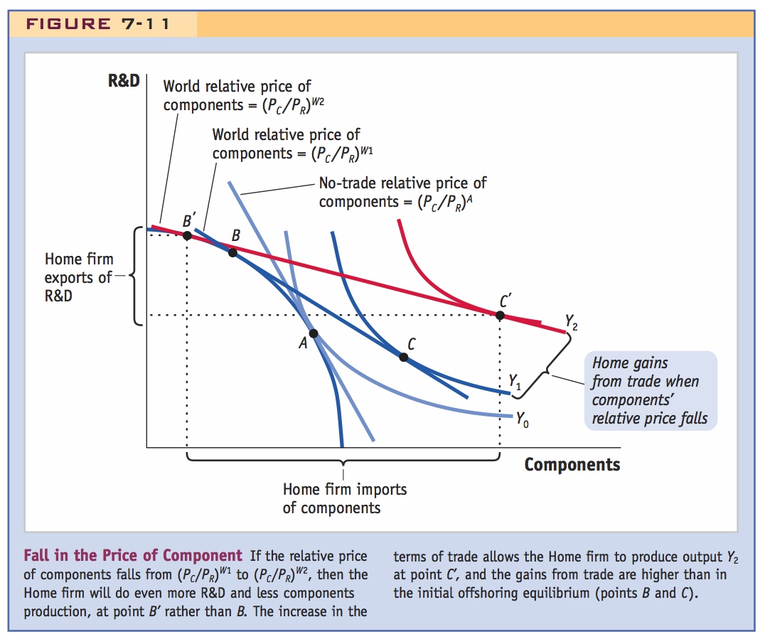
Fall in the Price of Components Turning to Figure 7-11, let the Home country start at the equilibrium with offshoring shown by points B and C. From that situation, suppose there is a fall in the relative price of component production. That price might fall, for instance, if the Foreign country improves its productivity in components, thereby lowering the price paid by Home for this service. Because components are being imported by Home, a fall in their price is a rise in the Home terms of trade, to (PR/PC)W2. Let us trace how this change in the terms of trade will affect the Home equilibrium.
If foreign becomes more productive in components, Home is even better off because the price of components will be lower.
Because of the fall in the relative price of components, the world price line shown in Figure 7-11 becomes flatter. Production will shift to point B′, and by exporting R&D and importing components along the world price line, the firm ends up at point C′. Production of the final good at point C′ is Y2, which exceeds the production Y1 in the initial equilibrium with offshoring.12 Thus, the Home firm enjoys greater gains from offshoring when the price of components falls. This is the first case considered by Samuelson, and it reinforces our conclusions that offshoring leads to overall gains.
218
Fall in the Price of R&D We also need to consider the second case identified by Samuelson, and that is when there is a fall in the price of R&D services rather than components. This is what Samuelson has in mind when he argues that offshoring might allow developing countries, such as India, to gain a comparative advantage in those activities in which the United States formerly had comparative advantage. As Indian companies like Wipro (an information technology services company headquartered in Bangalore) engage in more R&D activities, they are directly competing with American companies exporting the same services. So this competition can lower the world price of R&D services.
But if Foreign becomes more productive in R&D, then the relative price of components INCREASES, which tends to make Home worse off.
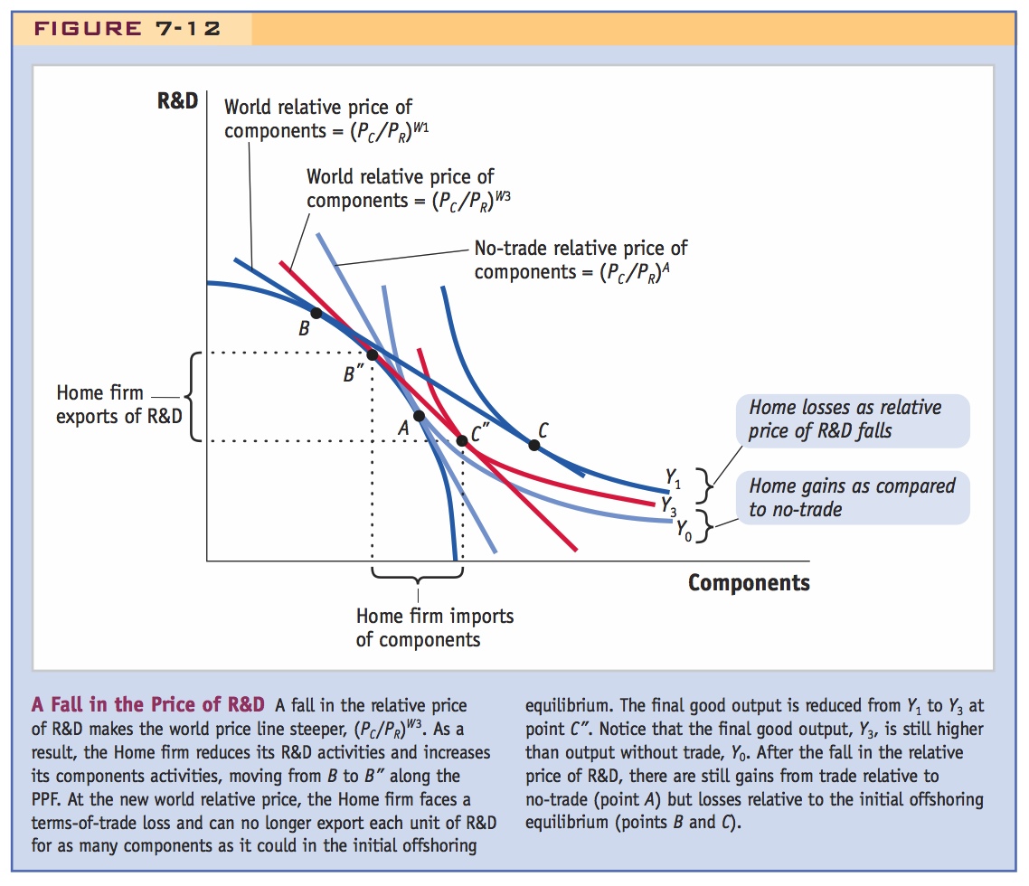
In Figure 7-12, we reproduce Figure 7-10, including the Home no-trade equilibrium at point A and the Home production point B with offshoring. Starting at point B, a fall in the world relative price of R&D will lead to a steeper price line (because the slope of the price line is the world relative price of components, which increases when PR falls). At the new price (PC/PR)W3, Home shifts production to point B″ and, by exporting R&D and importing components, moves to point C″. Notice that final output has fallen from Y1 to Y3. Therefore, the fall in the price of R&D services leads to losses for the Home firm. To explain where the losses are coming from, notice that Home is exporting R&D and importing components in the initial offshoring equilibrium (points B and C), so its terms of trade are the price of R&D divided by the price of components (PR/PC). With the fall in the price of R&D, the Home terms of trade have worsened, and Home is worse off compared with its initial offshoring equilibrium. Samuelson’s point is that the United States could be worse off if China or India becomes more competitive in, and lowers the prices of, the products that the United States itself is exporting, such as R&D services. This is theoretically correct. Although it may be surprising to think of the United States being in this position, the idea that a country will suffer when its terms of trade fall is familiar to us from developing-country examples (such as the Prebisch-Singer hypothesis) in earlier chapters.
So Samuelson is really just making a conventional terms-of-trade story, assuming that offshoring somehow raises Foreign productivity in R&D.
219
So offshoring is still a good thing overall, subject to the usual caveat that there are winners and losers. Notice that this is not nearly as provocative as the earlier quote in this section suggests.
Furthermore, notice that final output of Y3 is still higher than Y0, the no-offshoring output. Therefore, there are still Home gains from offshoring at C″ as compared with the no-trade equilibrium at A. It follows that Home can never be worse off with trade as compared with no trade. Samuelson’s point is that a country is worse off when its terms of trade fall, even though it is still better off than in the absence of trade. With the fall in the terms of trade, some factors of production will lose and others will gain, but in this case the gains of the winners are not enough to compensate the losses of the losers. Our simple model of offshoring illustrates Samuelson’s point.
The offshoring that occurred from the United States in the 1980s and the 1990s often concerned manufacturing activities. But today, the focus is frequently one of the newer forms of offshoring, the offshoring of business services to foreign countries. Business services are activities such as accounting, auditing, human resources, order processing, telemarketing, and after-sales service, like getting help with your computer. Firms in the United States are increasingly transferring these activities to India, where the wages of educated workers are much lower than in the United States. This is the sort of competition that Samuelson had in mind when he spoke of China and India improving their productivity and comparative advantage in activities that the United States already exports. The next application discusses the magnitude of service exports and also the changes in their prices.
No evidence this occurs . . .
The TOT for merchandise goods has improved for the U.S., so there are overall gains from offshoring there. The United States also has trade surpluses in many services, so the U.S. still seems to have a comparative advantage there too. But India may pose a competitive threat to the U.S. in computer and information services.
U.S. Terms of Trade and Service Exports
Because Samuelson’s argument is a theoretical one, the next step is to examine the evidence for the United States. If the United States has been facing competition in R&D and the other skill-intensive activities that we export, then we would expect the terms of trade to fall. Conversely, if the United States has been offshoring in manufacturing, then the opportunity to import lower-priced intermediate inputs should lead to a rise in the terms of trade.
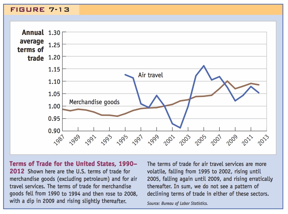
Merchandise Prices To evaluate these ideas, we make use of data on the terms of trade for the United States. In Figure 7-13, we first show the terms of trade for the United States for merchandise goods (excluding petroleum), which is the gold line.13 The terms of trade for goods fell from 1990 to 1994 but then rose to 2008, with a dip in 2009 and a slight rise thereafter. The overall improvement in the merchandise terms of trade shows that we are able to import intermediate inputs (and also import final goods) at lower prices over time. This rise in the terms of trade means that there are increasing gains from trade in merchandise goods for the United States.
220
Service Prices For trade in services, such as finance, insurance, and R&D, it is very difficult to measure their prices in international trade. These services are tailored to the buyer and, as a result, there are not standardized prices. For this reason, we do not have an overall measure of the terms of trade in services. There is one type of service, however, for which it is relatively easy to collect international prices: air travel. The terms of trade in air travel equal the price that foreigners pay for travel on U.S. airlines (a service export) divided by the price that Americans pay on foreign airlines (a service import). In Figure 7-13, we also show the U.S. terms of trade in air travel that are available since 1995. The terms of trade in air travel are quite volatile, falling from 1995 to 2002, rising until 2005, falling again until 2009, and rising erratically thereafter. For this one category of services, the terms of trade improvement from 2002 to 2005 indicates growing gains from trade for the United States, the same result we found for merchandise goods. Summing up, there is no evidence to date that the falling terms of trade that Samuelson is concerned about have occurred for the United States.
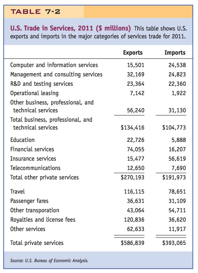
Service Trade What about other traded services? Although standard prices are not available, data on the amount of service exports and imports for the United States are collected annually. These data are shown in Table 7-2 for 2011. The United States runs a substantial surplus in services trade, with exports of $587 billion and imports of $393 billion. Categories of service exports that exceed imports include several types of business, professional, and technical services (but in computer and information services, the United States now runs a deficit); education (which is exported when a foreign student studies in the United States); financial services; travel; and royalties and license fees (which are collected from foreign firms when they use U.S. patents and trademarks or are paid abroad when we use foreign patents). The fact that exports exceed imports in many categories in Table 7-2 means that the United States has a comparative advantage in traded services. Indeed, the U.S. surplus in business, professional, and technical services is among the highest in the world, similar to that of the United Kingdom and higher than that of Hong Kong and India. London is a world financial center and competes with New York and other U.S. cities, which explains the high trade surplus of the United Kingdom, whereas Hong Kong is a regional hub for transportation and offshoring to China. The combined trade balance in computer and information services, insurance and financial services for the United States, the United Kingdom, and India since 1970 are graphed in Figure 7-14.

221
The U.S. surplus in these categories of services has been growing since about 1985, with an occasional dip, and exceeded the trade surplus of the United Kingdom, its chief competitor, up until about 2000. Since then the surpluses of the United Kingdom and of the United States have been quite similar. India’s surplus began growing shortly after 2000 and derives entirely from its exports of computer and information services. In 2010 the combined U.S. surplus in computers, insurance, and financial services ($122 billion) was three times larger than that of India ($37 billion), and about the same as of the United Kingdom ($108 billion).
What will these surpluses look like a decade or two from now? It is difficult to project, but notice in Figure 7-14 that in approximately 2000, as the Indian surplus began growing, the U.S. surplus dipped to become more similar to that of the United Kingdom. The Indian trade surplus is entirely due to its exports of computer and information services—a category in which the United States also has strong net exports. So even though the Indian trade surplus is still much smaller than that of the United States, it appears to pose a competitive challenge to the United States. It is at least possible that in a decade or two, India’s overall surplus in service exports could overtake that of the United States. Only time will tell whether the United States will eventually face the same type of competition from India in its service exports that it has already faced for many years from the United Kingdom.
222
. . . but things may change.