2 The Gains from Trade
1. Objectives: Review the gains from trade using consumer and producer surplus.
2. Consumer and Producer Surplus
Review of these concepts. Note that producer surplus can be interpreted as the return to a fixed factor, as the S-F model.
3. Home Welfare
Use the sum of consumer and producer surplus as a measure of welfare.
a. No Trade
Calculate Home welfare in autarky.
b. Free Trade for a Small Country
Suppose that the world price is less than the Home price in autarky. Quantity demanded increases, while quantity supplied decreases, so the Home imports the good.
c. Gains from Trade
Consumers gain more than producers lose, so there are gains from trade.
4. Home Import Demand Curve
Similar to Chapter 2: Lowering price raises quantity demand and lowers quantity supplied, so imports increase.
In earlier chapters, we demonstrated the gains from trade using a production possibilities frontier and indifference curves. We now instead demonstrate the gains from trade using Home demand and supply curves, together with the concepts of consumer surplus and producer surplus. You may already be familiar with these concepts from an earlier economics course, but we provide a brief review here.
Consumer and Producer Surplus
Don't assume the students are already familiar with these concepts.
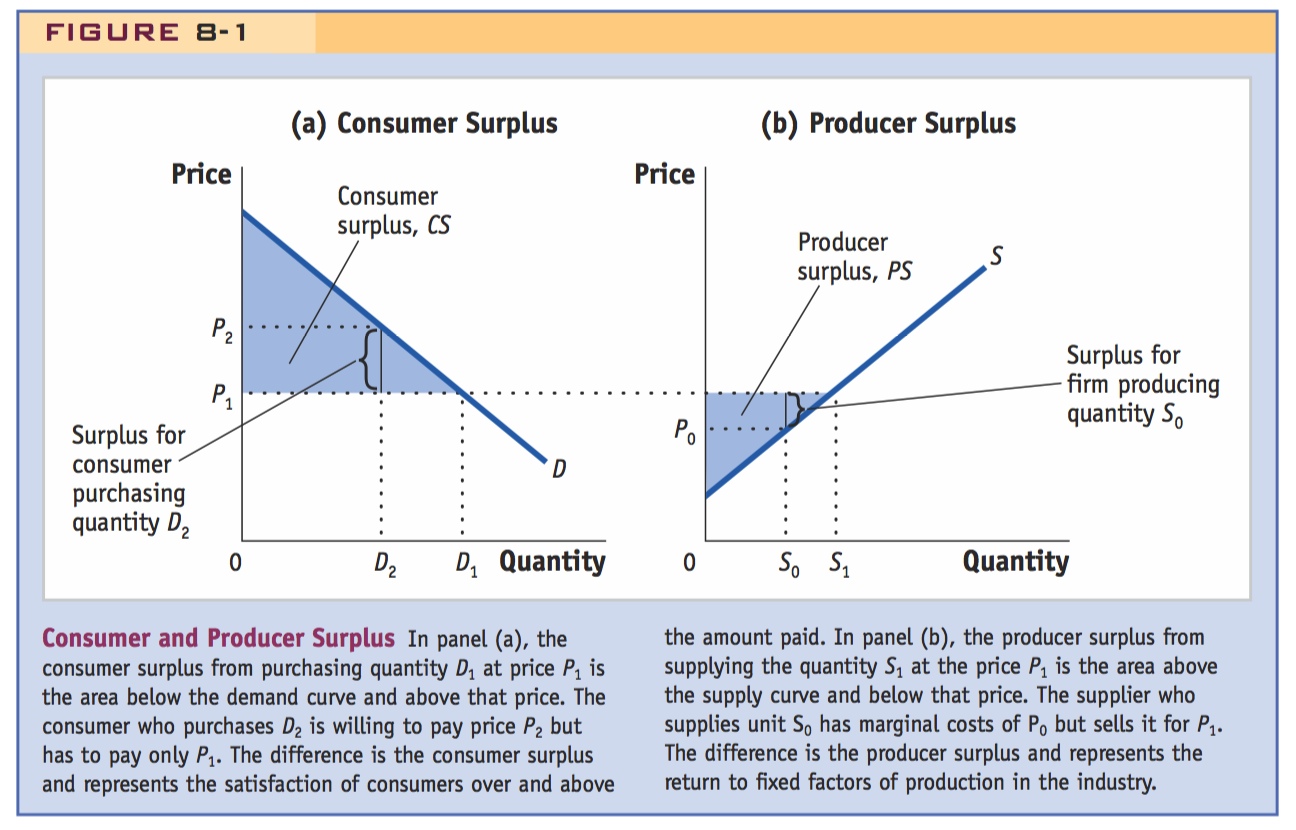
Suppose that Home consumers have the demand curve D in panel (a) of Figure 8-1 and face the price of P1. Then total demand is D1 units. For the last unit purchased, the consumer buying it values that unit at close to its purchase price of P1, so he or she obtains little or no surplus over the purchase price. But for all the earlier units purchased (from 0 to D1 units), the consumers valued the product at higher than its purchase price: the consumers’ willingness to pay for the product equals the height of the demand curve. For example, the person buying unit D2 would have been willing to pay the price of P2, which is the height of the demand curve at that quantity. Therefore, that individual obtains the surplus of (P2 − P1) from being able to purchase the good at the price P1.
237
SIDEBAR: Key Provisions of the GATT
Excerpts from the actual GATT rules, detailing the provisions described above.
Key Provisions of the GATT
ARTICLE I
General Most-Favoured-Nation Treatment
- With respect to customs duties…and with respect to all rules and formalities in connection with importation and exportation…any advantage, favour, privilege or immunity granted by any contracting party to any product originating in or destined for any other country shall be accorded immediately and unconditionally to the like product originating in or destined for the territories of all other contracting parties….
ARTICLE VI
Anti-Dumping and Countervailing Duties
- The contracting parties recognize that dumping, by which products of one country are introduced into the commerce of another country at less than the normal value of the products, is to be condemned if it causes or threatens material injury to an established industry…. [A] product is to be considered…less than its normal value, if the price of the product exported from one country to another
- is less than the comparable price…for the like product when destined for consumption in the exporting country, or,
- in the absence of such domestic price, is less than eitheri) the highest comparable price for the like product for export to any third country in the ordinary course of trade, or
ii) the cost of production of the product in the country of origin plus a reasonable addition for selling cost and profit….
ARTICLE XI
General Elimination of Quantitative Restrictions
- No prohibitions or restrictions other than duties, taxes or other charges, whether made effective through quotas, import or export licenses or other measures, shall be instituted or maintained by any contracting party on the importation of any product of the territory of any other contracting party or on the exportation or sale for export of any product destined for the territory of any other contracting party….
ARTICLE XVI
Subsidies
- If any contracting party grants or maintains any subsidy, including any form of income or price support, which operates directly or indirectly to increase exports of any product from, or to reduce imports of any product into, its territory, it shall notify the contracting parties in writing of the extent and nature of the subsidization. In any case in which it is determined that serious prejudice to the interests of any other contracting party is caused or threatened by any such subsidization, the contracting party granting the subsidy shall, upon request, discuss with the other contracting party…the possibility of limiting the subsidization.
ARTICLE XIX
Emergency Action on Imports of Particular Products
- If, as a result of unforeseen developments and of the effect of the obligations incurred by a contracting party under this Agreement, including tariff concessions, any product is being imported into the territory of that contracting party in such increased quantities and under such conditions as to cause or threaten serious injury to domestic producers in that territory of like or directly competitive products, the contracting party shall be free, in respect of such product, and to the extent and for such time as may be necessary to prevent or remedy such injury, to suspend the obligation in whole or in part or to withdraw or modify the concession….
ARTICLE XXIV
Territorial Application—Frontier Traffic—Customs Unions and Free-Trade Areas
- The contracting parties recognize the desirability of increasing freedom of trade by the development, through voluntary agreements, of closer integration between the economies of the countries party to such agreements. They also recognize that the purpose of a customs union or of a free-trade area should be to facilitate trade between the constituent territories and not to raise barriers to the trade of other contracting parties with such territories.
- Accordingly, the provisions of this Agreement shall not prevent [the formation of customs unions and free-trade areas, provided that:]
- …the duties [with outside parties] shall not on the whole be higher or more restrictive than the general incidence of the duties…prior to the formation….
Source: http://www.wto.org/english/docs_e/legal_e/gatt47_01_e.htm#articleI.
238
For each unit purchased before D1, the value that the consumer places on the product exceeds the purchase price of P1. Adding up the surplus obtained on each unit purchased, from 0 to D1, we can measure consumer surplus (CS) as the shaded region below the demand curve and above the price P1. This region measures the satisfaction that consumers receive from the purchased quantity D1, over and above the amount P1 · D1 that they have paid.
Panel (b) of Figure 8-1 illustrates producer surplus. This panel shows the supply curve of an industry; the height of the curve represents the firm’s marginal cost at each level of production. At the price of P1, the industry will supply S1. For the last unit supplied, the price P1 equals the marginal cost of production for the firm supplying that unit. But for all earlier units supplied (from 0 to S1 units), the firms were able to produce those units at a marginal cost less than the price P1. For example, the firm supplying unit S0 could produce it with a marginal cost of P0, which is the height of the supply curve at that quantity. Therefore, that firm obtains the producer surplus of (P1 − P0) from being able to sell the good at the price P1.
239
Remind them again of the difference between accounting profit and economic profit.
For each unit sold before S1, the marginal cost to the firm is less than the sale price of P1. Adding up the producer surplus obtained for each unit sold, from 0 to S1, we obtain producer surplus (PS) as the shaded region in panel (b) above the supply curve and below the price of P1. It is tempting to think of producer surplus as the profits of firms, because for all units before S1, the marginal cost of production is less than the sale price of P1. But a more accurate definition of producer surplus is that it equals the return to fixed factors of production in the industry. That is, producer surplus is the difference between the sales revenue P1 · S1 and the total variable costs of production (i.e., wages paid to labor and the costs of intermediate inputs). If there are fixed factors such as capital or land in the industry, as in the specific-factors model we studied in Chapter 3, then producer surplus equals the returns to these fixed factors of production. We might still loosely refer to this return as the “profit” earned in the industry, but it is important to understand that producer surplus is not monopoly profit, because we are assuming perfect competition (i.e., zero monopoly profits) throughout this chapter.3
Home Welfare
To examine the effects of trade on a country’s welfare, we consider once again a world composed of two countries, Home and Foreign, with each country consisting of producers and consumers. Total Home welfare can be measured by adding up consumer and producer surplus. As you would expect, the greater the total amount of Home welfare, the better off are the consumers and producers overall in the economy. To measure the gains from trade, we will compare Home welfare in no-trade and freetrade situations.
Use this as an opportunity to discuss the First Welfare Theorem: Demonstrate that the equilibrium price maximizes the sum of consumer and producer surplus, so that the "pie" is as big as possible.
This, in turn, is a good place to digress to talk about Pareto optimality and the gains from trade.
Work through a numerical example, so they get used to calculating these areas.
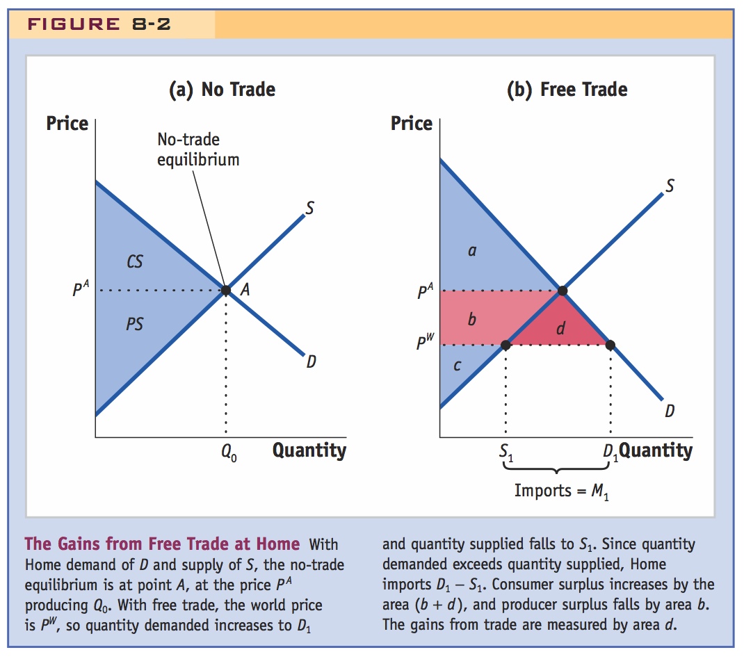
No Trade In panel (a) of Figure 8-2, we combine the Home demand and supply curves in a single diagram. The no-trade equilibrium occurs at the autarky price of PA, where the quantity demanded equals the quantity supplied, of Q0. Consumer surplus is the region above the price of PA and below the demand curve, which is labeled as CS in panel (a) and also shown as area a in panel (b). Producer surplus is the area below the price of PA and above the supply curve, which is labeled as PS in panel (a) and also shown as area (b + c) in panel (b). So the sum of consumer surplus and producer surplus is the area between the demand and supply curves, or CS + PS = area (a + b + c). That area equals Home welfare in the market for this good in the absence of international trade.
The text does this later, but let the students think through what would happen if the world price were greater than the domestic autarky price.
For future reference, ask students what happens to imports if world prices decrease.
Again, let students show this themselves.
Free Trade for a Small Country Now suppose that Home can engage in international trade for this good. As we have discussed in earlier chapters, the world price PW is determined by the intersection of supply and demand in the world market. Generally, there will be many countries buying and selling on the world market. We will suppose that the Home country is a small country, by which we mean that it is small in comparison with all the other countries buying and selling this product. For that reason, Home will be a price taker in the world market: it faces the fixed world price of PW, and its own level of demand and supply for this product has no influence on the world price. In panel (b) of Figure 8-2, we assume that the world price PW is below the Home no-trade price of PA. At the lower price, Home demand will increase from Q0 under no trade to D1, and Home supply will decrease from Q0 under no trade to S1. The difference between D1 and S1 is imports of the good, or M1 = D1 − S1. Because the world price PW is below the no-trade price of PA, the Home country is an importer of the product at the world price. If, instead, PW were above PA, then Home would be an exporter of the product at the world price.
240
Have the students develop their own numerical example and calculate PS, CS, and the gains from trade.
Gains from Trade Now that we have established the free-trade equilibrium at price PW, it is easy to measure Home welfare as the sum of consumer and producer surplus with trade, and compare it with the no-trade situation. In panel (b) of Figure 8-2, Home consumer surplus at the price PW equals the area (a + b + d), which is the area below the demand curve and above the price PW. In the absence of trade, consumer surplus was the area a, so the drop in price from PA to PW has increased consumer surplus by the amount (b + d). Home consumers clearly gain from the drop in price.
Home firms, on the other hand, suffer a decrease in producer surplus from the drop in price. In panel (b), Home producer surplus at the price PW equals the area c, which is the area above the supply curve and below the price PW. In the absence of trade, producer surplus was the area (b + c), so the drop in price from PA to PW has decreased producer surplus by the amount b. Home firms clearly lose from the drop in price.
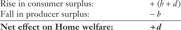
Comparing the gains of consumers, (b + d), with the losses of producers, area b, we see that consumers gain more than the producers lose, which indicates that total Home welfare (the sum of consumer surplus and producer surplus) has gone up. We can calculate the total change in Home welfare due to the opening of trade by adding the changes in consumer surplus and producer surplus:
241
Return to the theme that free trade is a potential Pareto improvement, but has distributional effects.
The area d is a measure of the gains from trade for the importing country due to free trade in this good. It is similar to the gains from trade that we have identified in earlier chapters using the production possibilities frontier and indifference curves, but it is easier to measure: the triangle d has a base equal to free-trade imports M1 = D1 − S1, and a height that is the drop in price, PA − PW, so the gains from trade equal the area of the triangle,  · (PA − PW) · M1. Of course, with many goods being imported, we would need to add up the areas of the triangles for each good and take into account the net gains on the export side to determine the overall gains from trade for a country. Because gains are positive for each individual good, after summing all imported and exported goods, the gains from trade are still positive.
Home Import Demand Curve
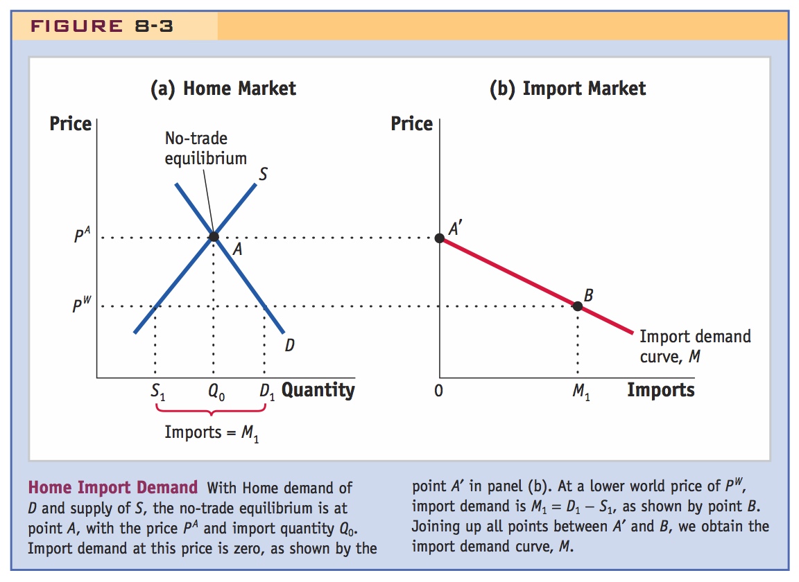
Before introducing a tariff, we use Figure 8-3 to derive the import demand curve, which shows the relationship between the world price of a good and the quantity of imports demanded by Home consumers. We first derived this curve in Chapter 2, for the Ricardian model. We now briefly review the derivation of the import demand curve before analyzing the effect of an import tariff on prices and welfare.
242
In panel (a) of Figure 8-3, we again show the downward-sloping Home demand curve (D) and the upward-sloping Home supply curve (S). The no-trade equilibrium is at point A, which determines Home’s no-trade equilibrium price PA, and its no-trade equilibrium quantity of Q0. Because quantity demanded equals quantity supplied, there are zero imports of this product. Zero imports is shown as point A′ in panel (b).
Now suppose the world price is at PW, below the no-trade price of PA. At the price of PW, the quantity demanded in Home is D1, but the quantity supplied by Home suppliers is only S1. Therefore, the quantity imported is M1 = D1 − S1, as shown by the point B in panel (b). Joining points A′ and B, we obtain the downward-sloping import demand curve M.
If you haven't done so already, let students think through this themselves as an exercise.
Notice that the import demand curve applies for all prices below the no-trade price of PA in Figure 8-3. Having lower prices leads to greater Home demand and less Home supply and, therefore, positive imports. What happens if the world price is above the no-trade price? In that case, the higher price would lead to greater Home supply and less Home demand, so Home would become an exporter of the product.