4 Import Tariffs for a Large Country
If the country is large, the tariff may alter the world price.
This may actually make the country better off.
1. Foreign Export Supply
Foreign export is no longer perfectly elastic if Home is large. Derive a positively sloped Foreign export supply curve. World price is determined where the Home import demand and Foreign export supply intersect.
2. Effect of the Tariff
Foreign export supply curve upwards vertically by the amount of the tariff. Foreigners receive a lower world price, while the Home price increases by less than the tariff: Part of the incidence of the tariff is being shifted to Foreign.
a. Terms of Trade: The tariff has improved Home’s terms of trade (TOT), which tends to make Home better off.
b. Home Welfare: There are still losses in consumer and gain in producer surplus, but now there is also a terms-of-trade gain, equal to the fall in world price x imports. The tariff improves Home’s welfare if the TOT gain exceeds the losses in consumer and producer surplus.
c. Foreign and World Welfare: The TOT gain to Home is a loss to Foreign: it now sells less at lower prices. A tariff imposed by a large country is a “beggar thy neighbor” policy. It redistributes income from Foreign to Home, and creates a world deadweight loss.
d. Optimal Tariff for a Large Importing Country: What tariff would maximize Home welfare? Starting from a small tariff, increasing it will raise welfare because the TOT gain exceeds the deadweight loss. For very large tariffs the converse is true, and welfare falls below that in autarky. Therefore, there must exist a tariff that maximizes Home’s welfare.
e. Optimal Tariff Formula: Intuitively, the magnitude of the TOT gain depends upon how much the world price falls, which is determined by the elasticity of Foreign export supply. In fact, the optimal tariff is equal to the reciprocal of the elasticity of Foreign export supply.
Under the small-country assumption that we have used so far, we know for sure that the deadweight loss is positive; that is, the importing country is always harmed by the tariff. The small-country assumption means that the world price PW is unchanged by the tariff applied by the importing country. If we consider a large enough importing country or a large country, however, then we might expect that its tariff will change the world price. In that case, the welfare for a large importing country can be improved by a tariff, as we now show.
Foreign Export Supply
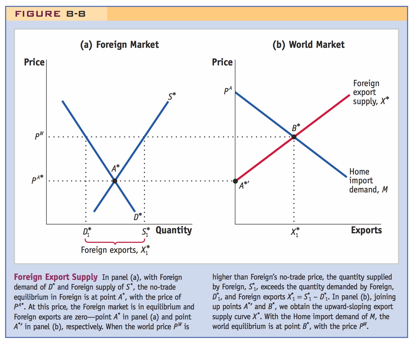
If the Home country is large, then we can no longer assume that it faces a Foreign export supply curve X* that is horizontal at the given world price PW. Instead, we need to derive the Foreign export supply curve using the Foreign market demand and supply curves. In panel (a) of Figure 8-8, we show the Foreign demand curve D* and supply curve S*. These intersect at the point A*, with a no-trade equilibrium price of PA*. Because Foreign demand equals supply at that price, Foreign exports are zero, which we show by point A*′ in panel (b), where we graph Foreign exports against their price.
257
Now suppose the world price PW is above the Foreign no-trade price of PA*. At the price of PW, the Foreign quantity demanded is lower, at  in panel (a), but the quantity supplied by Foreign firms is larger, at
  . Because Foreign supply exceeds demand, Foreign will export the amount
  = − at the price of PW, as shown by the point B* in panel (b). Drawing a line through points A*′ and B*, we obtain the upward-sloping Foreign export supply curve X*.
We can then combine the Foreign export supply curve X* and Home import demand curve M, which is also shown in panel (b). They intersect at the price PW, the world equilibrium price. Notice that the Home import demand curve starts at the no-trade price PA on the price axis, whereas the Foreign export supply curve starts at the price PA*. As we have drawn them, the Foreign no-trade price is lower, PA* < PA. In Chapters 2 to 5 of this book, a country with comparative advantage in a good would have a lower no-trade relative price and would become an exporter when trade was opened. Likewise, in panel (b), Foreign exports the good since its no-trade price PA* is lower than the world price, and Home imports the good since its no-trade price PA is higher than the world price. So the world equilibrium illustrated in panel (b) is similar to that in some of the trade models presented in earlier chapters.
Effect of the Tariff
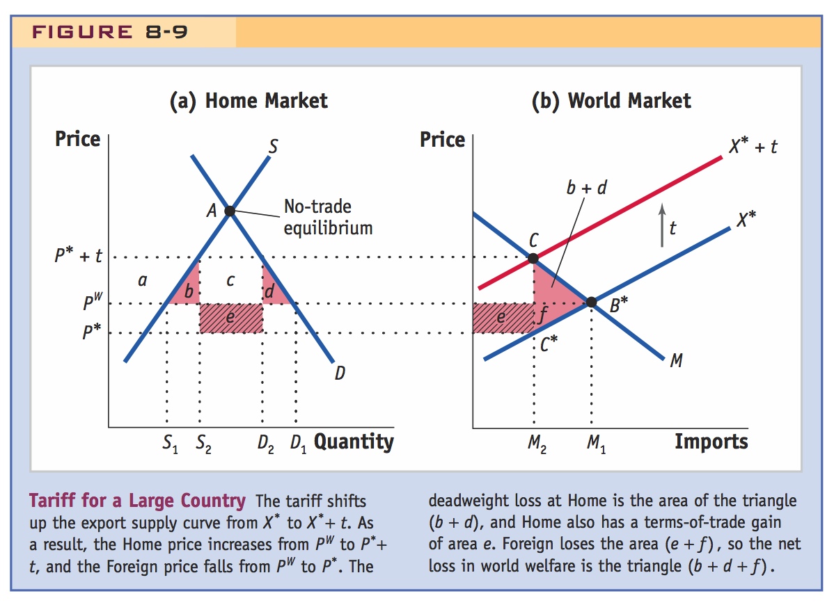
In panel (b) of Figure 8-9, we repeat the Home import demand curve M and Foreign export supply curve X*, with the world equilibrium at B*. When Home applies a tariff of t dollars, the cost to Foreign producers of supplying the Home market is t more than it was before. Because of this increase in costs, the Foreign export supply curve shifts up by exactly the amount of the tariff, as shown in panel (b) with the shift from X* to X* + t. The X* + t curve intersects import demand M at point C, which establishes the Home price (including the tariff) paid by consumers. On the other hand, the Foreign exporters receive the net-of-tariff price, which is directly below the point C by exactly the amount t, at point C*. Let us call the price received by Foreign exporters P*, at point C*, which is the new world price.
Perhaps first review the analysis of an excise tax in a competitive market, since this is an exercise in incidence. Doing so will also establish the principle that the effects are the same regardless of which side of the market the tax is levied.
The important feature of the new equilibrium is that the price Home pays for its imports, P* + t, rises by less than the amount of the tariff t as compared with the initial world price PW. The reason that the Home price rises by less than the full amount of the tariff is that the price received by Foreign exporters, P*, has fallen as compared with the initial world price PW. So, Foreign producers are essentially “absorbing” a part of the tariff, by lowering their price from PW (in the initial free-trade equilibrium) to P* (after the tariff).
Use the "irrelevance of who pays" principle mentioned above to argue the effects of the tariff would be the same regardless of if foreign exporters paid it to the government or if domestic consumers had to pay it. Have students shift Home import demand rather than export supply, and let them compare.
In sum, we can interpret the tariff as driving a wedge between what Home consumers pay and what Foreign producers receive, with the difference (of t) going to the Home government. As is the case with many taxes, the amount of the tariff (t) is shared by both consumers and producers.
258
Terms of Trade In Chapter 2, we defined the terms of trade for a country as the ratio of export prices to import prices. Generally, an improvement in the terms of trade indicates a gain for a country because it is either receiving more for its exports or paying less for its imports. To measure the Home terms of trade, we want to use the net-of-tariff import price P* (received by Foreign firms) since that is the total amount transferred from Home to Foreign for each import. Because this price has fallen (from its initial world price of PW), it follows that the Home terms of trade have increased. We might expect, therefore, that the Home country gains from the tariff in terms of Home welfare. To determine whether that is the case, we need to analyze the impact on the welfare of Home consumers, producers, and government revenue, which we do in Figure 8-9.
Home Welfare In panel (a), the Home consumer price increases from PW to P* + t, which makes consumers worse off. The drop in consumer surplus is represented by the area between these two prices and to the left of the demand curve D, which is shown by (a + b + c + d). At the same time, the price received by Home firms rises from PW to P* + t, making Home firms better off. The increase in producer surplus equals the area between these two prices, and to the left of the supply curve S, which is the amount a. Finally, we also need to keep track of the changes in government revenue. Revenue collected from the tariff equals the amount of the tariff (t) times the new amount of imports, which is M2 = D2 − S2. Therefore, government revenue equals the area (c + e) in panel (a).
By summing the change in consumer surplus, producer surplus, and government revenue, we obtain the overall impact of the tariff in the large country, as follows:
259
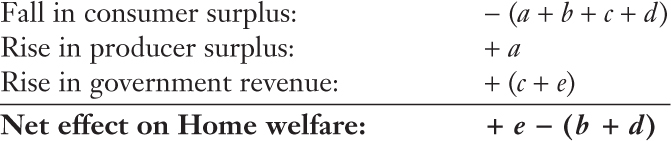
The triangle (b + d) is the deadweight loss due to the tariff (just as it is for a small country). But for the large country, there is also a source of gain—the area e—that offsets this deadweight loss. If e exceeds (b + d), then Home is better off due to the tariff; if e is less than (b + d), then Home is worse off.
Notice that the area e is a rectangle whose height is the fall in the price that Foreign exporters receive, the difference between PW and P*. The base of this rectangle equals the quantity of imports, M2. Multiplying the drop in the import price by the quantity of imports to obtain the area e, we obtain a precise measure of the terms-of-trade gain for the importer. If this terms-of-trade gain exceeds the deadweight loss of the tariff, which is (b + d), then Home gains from the tariff.
Thus, we see that a large importer might gain by the application of a tariff. We can add this to our list of reasons why countries use tariffs, in addition to their being a source of government revenue or a tool for political purposes. However, for the large country, any net gain from the tariff comes at the expense of the Foreign exporters, as we show next.
Foreign and World Welfare While Home might gain from the tariff, Foreign, the exporting country, definitely loses. In panel (b) of Figure 8-9, the Foreign loss is measured by the area (e + f). We should think of (e + f) as the loss in Foreign producer surplus from selling fewer goods to Home at a lower price. Notice that the area e is the terms-of-trade gain for Home but an equivalent terms-of-trade loss for Foreign; Home’s gain comes at the expense of Foreign. In addition, the large-country tariff incurs an extra deadweight loss of f in Foreign, so the combined total outweighs the benefits to Home. For this reason, we sometimes call a tariff imposed by a large country a “beggar thy neighbor” tariff.
Adding together the change in Home welfare and Foreign welfare, the area e cancels out and we are left with a net loss in world welfare of (b + d + f), the triangle in panel (b). This area is a deadweight loss for the world. The terms-of-trade gain that Home has extracted from the Foreign country by using a tariff comes at the expense of the Foreign exporters, and in addition, there is an added world deadweight loss. The fact that the large-country tariff leads to a world deadweight loss is another reason that most economists oppose the use of tariffs.
Its OWN welfare.
Optimal Tariff for a Large Importing Country We have found that a large importer might gain by the application of tariffs, but have yet to determine what level of tariff a country should apply in order to maximize welfare. It turns out there is a shortcut method we can use to evaluate the effect of the tariff on the welfare of a large importing country. The shortcut method uses the concept of the optimal tariff.
The optimal tariff is defined as the tariff that leads to the maximum increase in welfare for the importing country. For a large importing country, a small tariff initially increases welfare because the terms-of-trade gain exceeds the deadweight loss. That is, the area of the rectangle e in panel (a) of Figure 8-9 exceeds the area of the triangle (b + d) in panel (b) when the tariff is small enough. The reason for this is that both the height and base of the triangle (b + d) shrink to zero when the tariff is very small, so the area of the triangle is very small indeed; but for the rectangle e, only the height shrinks to zero when the tariff is small, so the area of the rectangle exceeds that of the triangle. By this mathematical reasoning, the Home gains are positive—e > (b + d)—when the Home tariff is sufficiently small.
260
In Figure 8-10, we graph Home welfare against the level of the tariff. Free trade is at point B, where the tariff is zero. A small increase in the tariff, as we have just noted, leads to an increase in Home welfare (because the terms-of-trade gain exceeds the deadweight loss). Therefore, starting at point B, the graph of Home welfare must be upward-sloping. But what if the tariff is very large? If the tariff is too large, then welfare will fall below the free-trade level of welfare. For example, with a prohibitive tariff so high that no imports are purchased at all, then the importer’s welfare will be at the no-trade level, shown by point A. So while the graph of welfare must be increasing for a small tariff from point B, as the tariff increases, welfare eventually falls past the free-trade level at point B′ to the no-trade welfare at point A.
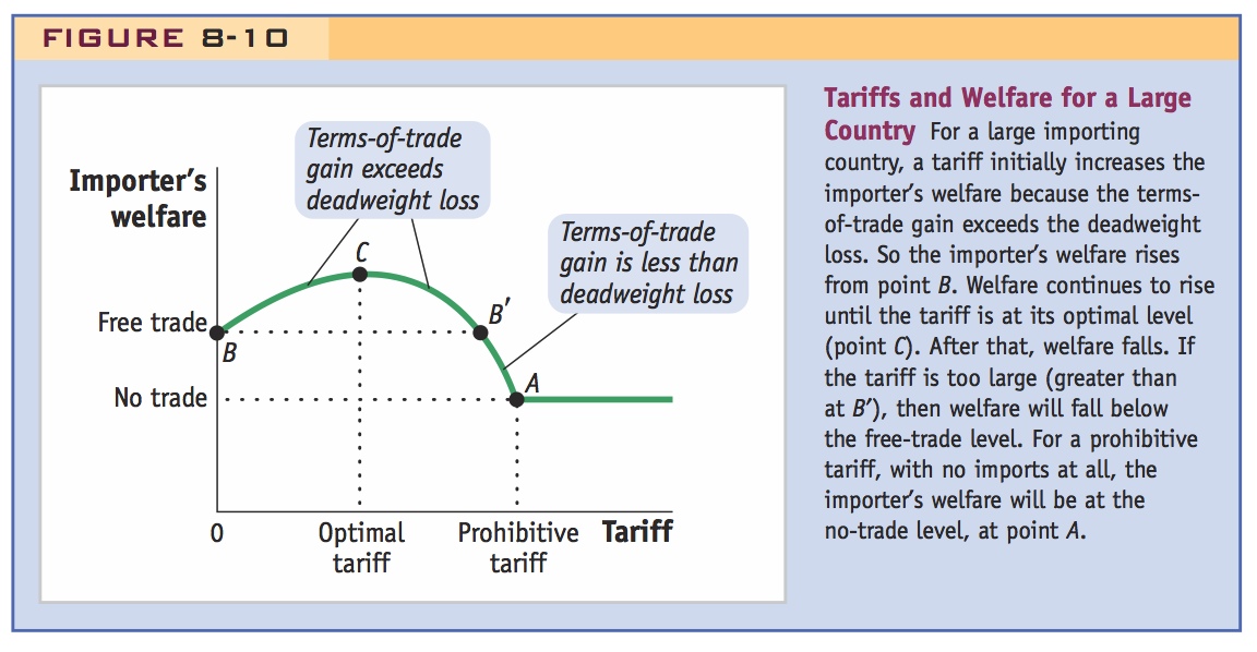
Given that points B and A are both on the graph of the importer’s welfare (for free trade and no trade, respectively) and that welfare must be rising after point B, it follows that there must be a highest point of welfare, shown by point C. At this point, the importer’s welfare is highest because the difference between the terms-of-trade gain and deadweight loss is maximized. We will call the tariff at that point the “optimal tariff.” For increases in the tariff beyond its optimal level (i.e., between points C and A), the importer’s welfare falls because the deadweight loss due to the tariff overwhelms the terms-of-trade gain. But whenever the tariff is below its optimal level, between points B and C, then welfare is higher than its free-trade level because the terms-of-trade gain exceeds the deadweight loss.
Optimal Tariff Formula It turns out that there is a simple formula for the optimal tariff. The formula depends on the elasticity of Foreign export supply, which we call  . Recall that the elasticity of any supply curve is the percentage increase in supply caused by a percentage increase in price. Likewise, the elasticity of the Foreign export supply curve is the percentage change in the quantity exported in response to a percent change in the world price of the export. If the export supply curve is very steep, then there is little response of the quantity supplied, and so the elasticity is low. Conversely, if the export supply curve is very flat, there is a large response of the quantity supplied due to a change in the world price, and so is high. Recall also that a small importing country faces a perfectly horizontal, or perfectly elastic, Foreign export supply curve, which means that the elasticity of Foreign export supply is infinite.
261
Using the elasticity of Foreign export supply, the optimal tariff equals

That is, the optimal tariff (measured as a percentage) equals the inverse of the elasticity of Foreign export supply. For a small importing country, the elasticity of Foreign export supply is infinite, and so the optimal tariff is zero. That result makes sense, since any tariff higher than zero leads to a deadweight loss for the importer (and no terms-of-trade gain), so the best tariff to choose is zero, or free trade.
For a large importing country however, the Foreign export supply is less than infinite, and we can use this formula to compute the optimal tariff. As the elasticity of Foreign export supply decreases (which means that the Foreign export supply curve is steeper), the optimal tariff is higher. The reason for this result is that with a steep Foreign export supply curve, Foreign exporters will lower their price more in response to the tariff.13 For instance, if decreases from 3 to 2, then the optimal tariff increases from  = 33% to
  = 50%, reflecting the fact that Foreign producers are willing to lower their prices more, taking on a larger share of the tariff burden. In that case, the Home country obtains a larger terms-of-trade increase and hence the optimal level of the tariff is higher.
Is the U.S. large enough in the steel market to have benefited from the steel tariffs? Use estimates of export supplies to the U.S. for three steel products to calculate the optimal tariffs. For two of the three, the actual tariff raised welfare. But this was at the expense of foreign exporters.
U.S. Tariffs on Steel Once Again
Let us return to the U.S. tariff on steel, and reevaluate the effect on U.S. welfare in the large-country case. The calculation of the deadweight loss that we did earlier in the application assumed that the United States was a small country, facing fixed world prices for steel. In that case, the 30% tariff on steel was fully reflected in U.S. prices, which rose by 30%. But what if the import prices for steel in the United States did not rise by the full amount of the tariff? If the United States is a large enough importer of steel, then the Foreign export price will fall and the U.S. import price will rise by less than the tariff. It is then possible that the United States gained from the tariff.
To determine whether the United States gained from the tariff on steel products, we can compute the deadweight loss (area b + d) and the terms-of-trade gain (area e) for each imported steel product using the optimum tariff formula.
Optimal Tariffs for Steel Let us apply this formula to the U.S. steel tariffs to see how the tariffs applied compare with the theoretical optimal tariff. In Table 8-2, we show various steel products along with their respective elasticities of export supply to the United States. By taking the inverse of each export supply elasticity, we obtain the optimal tariff. For example, alloy steel flat-rolled products (the first item) have a low export supply elasticity, 0.27, so they have a very high optimal tariff of 1/0.27 = 3.7 = 370%. In contrast, iron and nonalloy steel flat-rolled products (the last item) have a very high export supply elasticity of 750, so the optimal tariff is 1/750 ≈ 0%. Products between these have optimal tariffs ranging from 1% to 125%.

262
In the final column of Table 8-2, we show the actual tariffs that were applied to these products. For alloy steel flat-rolled products (the first item), the actual tariff was 30%, which is far below the optimal tariff. That means the terms-of-trade gain for that product was higher than the deadweight loss: the tariff is on the portion of the welfare graph between B and C in Figure 8-10, and U.S. welfare is above its free-trade level. The same holds for iron and steel bars, rods, angles, and shapes, for which the tariffs of 15% to 30% are again less than their optimal level, so the United States obtains a terms-of-trade gain that exceeds the deadweight loss. However, for iron and steel tubes, pipes, and fittings, the U.S. tariffs were 13% to 15%, but the optimal tariff for that product was only 1%. Because of the very high elasticity of export supply, the United States has practically no effect on the world price, so the deadweight loss for that product exceeds the terms-of-trade gain.
To summarize, for the three product categories in Table 8-2 to which the United States applied tariffs, in two products the terms-of-trade gain exceeded the deadweight loss, so U.S. welfare rose due to the tariff, but in a third case the deadweight loss was larger, so U.S. welfare fell due to the tariff. The first two products illustrate the large-country case for tariffs, in which the welfare of the importer can rise because of a tariff, whereas the third product illustrates the small-country case, in which the importer loses from the tariff.
From the information given in Table 8-2, we do not know whether the United States gained or lost overall from the steel tariffs: that calculation would require adding up the gains and losses due to the tariff over all imported steel products, which we have not done. But in the end, we should keep in mind that any rise in U.S. welfare comes at the expense of exporting countries. Even if there were an overall terms-of-trade gain for the United States when adding up across all steel products, that gain would be at the expense of the European countries and other steel exporters. As we have already discussed, the steel exporters objected to the U.S. tariffs at the WTO and were entitled to apply retaliatory tariffs of their own against U.S. products. If these tariffs had been applied, they would have eliminated and reversed any U.S. gain. By removing the tariffs in less than two years, the United States avoided a costly tariff war. Indeed, that is one of the main goals of the WTO: by allowing exporting countries to retaliate with tariffs, the WTO prevents importers from using optimal tariffs to their own advantage. In a later chapter, we show more carefully how such a tariff war will end up being costly to all countries involved.
263
And they might retaliate