3 Debt and Default
Sovereign default has a long history. Advanced countries rarely default now, although some debtor countries in Europe have been at risk in the recent crisis. However, sovereign default is a recurrent problem among developing countries, which seem to get into trouble at much lower debt levels than advanced countries.
1. A Few Peculiar Facts About Sovereign Default
Unlike private debtors, sovereign states cannot be forced to repay their debts. Sovereign default is therefore a rational choice. What are the benefits and costs of defaulting? The benefit is keeping the money. There are two types of costs: (1) The country may be excluded from credit markets. However, the cost may be low if the exclusion period is short. (2) There may be broader macroeconomic costs, including losses in investment, trade, and output, as well as risk premia, exchange rate crisis, and banking crises.
a. Summary
Sovereign default involves a rational comparison of costs and benefits. We will develop a simple model to explain the decision, explain why default can occur even at low amounts of debt, and why lenders might continue to lend to defaulting countries.
2. A Model of Default, Part One: The Probability of Default
a. Assumptions
Ignore investment in order to focus on consumption smoothing. Assume output fluctuates between a high value, Y̅ and low value, Y̅ - V ; the difference V is a measure of the volatility of output. The government takes out a loan L before output is known; the interest rate is rL paid after output is realized. Questions: (1) What are the terms of the loan contract? (2) When will the country default?
b. The Borrower Chooses Default Versus Repayment
Assume the cost of repayment is the loss of a fraction c on output. Then the country will repay as long as consumption after repayment > consumption with nonrepayment. This implies a threshold output YT = (1 + rL)/c above which the country will repay. Depict this graphically; relate the size of the repayment region to the default region as the probability p of repayment.
c. An Increase in the Debt Burden
Suppose that the burden (1 + rL) increases. This raises the threshold YT so that the probability of repayment decreases. Notice that if the burden increases enough, the probability of repayment could drop to zero. Conversely, the probability could increase to 1 if the burden falls enough.
d. An Increase in Volatility of Output
If V increases, the threshold is the same, but the range of lower values of output has increased. This makes repayment less likely because the default region is larger; if V increases enough default could occur with probability 1.
e. The Lender Chooses the Lending Rate
To break even, a competitive lender must charge an interest rate that will allow it to break even. It will set rL to equate the expected revenue per dollar lent to the expected borrowing costs: p(1 + rL) = 1 = r where r is the world interest rate. So the lender charges a risk premium.
In the chapter on the gains from financial globalization, when global capital markets work well, they can deliver gains in the form of consumption smoothing and investment efficiency. Yet international financial relations are often disrupted by sovereign default, which occurs when a sovereign government (i.e., one that is autonomous or independent) fails to meet its legal obligations to make payments on debt held by foreigners.
Sovereign default has a long history. Perhaps the first recorded default was in the fourth century BC, when Greek municipalities defaulted on loans from the Delos Temple.14 Many of today’s advanced countries have defaulted in the past. In 1343 a war-weary Edward III of England defaulted on short-term loans which ruined the major merchant banks of Florence, Italy. In 1557, Phillip II of Spain defaulted on short-term loans principally from South German bankers.15 Spain defaulted six more times before 1800 and another seven times in the nineteenth century. France defaulted eight times between 1558 and the Revolution in 1789. A group of German states, Portugal, Austria, and Greece defaulted at least four times each in the 1800s, and across Europe as a whole, there were at least 46 sovereign defaults between 1501 and 1900.16 The United States has maintained a clean sheet during its brief existence, although several U.S. states defaulted when they were emerging markets in the 1800s.17
475
Emphasize that this is mostly a problem of developing countries.
The advanced countries of today tend not to default, although the large debts they have incurred during the Global Financial Crisis may put some of them at greater risk (from 2010 to 2013 countries such as Ireland, Portugal, Spain, Italy, Slovenia, and Cyprus have been under strain, and Greece actually defaulted). In contrast, default has been, and remains, a recurring problem in emerging markets and developing countries. One count shows that countries such as Argentina, Brazil, Mexico, Turkey, and Venezuela have defaulted between five and nine times since 1824 (and at least once since 1980) and have spent 30% of the time failing to meet their financial obligations. Another count lists 48 sovereign defaults in the period from 1976 to 1989, many in Latin America but others dotted throughout the world, and 16 more in the period from 1998 to 2002, including headline crises in Russia (1998) and Argentina (2002).18
One of the most puzzling aspects of the default problem is that emerging markets and developing countries often get into default trouble at much lower levels of debt than advanced countries. Yet default is a serious macroeconomic and financial problem for these countries. Because they attract so few financial flows of other kinds, government debt constitutes a large share (more than 30%) of these nations’ external liabilities.19
To understand the workings of sovereign debt and defaults, we must first look at some of the peculiar characteristics of this form of borrowing.
A Few Peculiar Facts About Sovereign Debt
The crucial fact
The first important fact about sovereign debt is that debtors are almost never forced to pay. Using the military to enforce repayment is always costly, and is certainly out of fashion in the modern world. Legal actions are also largely futile: when developing country debt is issued in a foreign jurisdiction (e.g., in London or New York), there is practically no legal way to enforce a claim against a sovereign nation, and the recent increase in sovereign default litigation has done very little to change this state of affairs.20
476
Say that, being economists, we address the question by comparing costs and benefits. Then list both.
The repayment of a sovereign debt is thus a matter of choice for the borrowing government. Economists are therefore inclined to look for a rational explanation in which default is triggered by economic conditions: how painful does repayment have to become before default occurs?
To answer this question, we must evaluate the costs and benefits of default. The benefits are clear: no repayment means the country gets to keep all that money. Are there costs? While not as apparent as the benefits, there must be costs to default—if there were no costs, countries would never pay their debts, and, as a result, no lending would happen in the first place! Thus economists (ignoring sentimental motives for repayment such as honor and honesty) have focused on two types of costs that act as a “punishment” for defaulters and provide the incentive for nations to repay their debts.21
- Financial market penalties. Empirical evidence shows that debtors are usually excluded from credit markets for some time after a default. This exclusion could expose them to greater consumption risk and other disadvantages. However, economic theory casts doubt on whether avoiding these costs is enough of an incentive to repay the loans. Repayment is less likely when the exclusion period is short or when borrowers have other ways to smooth consumption (such as investing previously borrowed wealth, purchasing insurance, or going to a different set of financial intermediaries).
- Broader macroeconomic costs. These could include lost investment, lost trade, or lost output arising from adverse financial conditions in the wake of a default. These adverse conditions include higher risk premiums, credit contractions, exchange rate crises, and banking crises. If these costs are high enough, they can encourage nations to repay, even if financial market costs are insufficient.
Summary Sovereign debt is a contingent claim on a nation’s assets: governments will repay depending on whether it is more beneficial to repay than to default. With a simple model of how a country makes the decision to default, we can better understand why borrowers default some of the time and repay some of the time; what ultimately causes these contingent outcomes; why some borrowers get into default trouble even at low levels of debt, while others do not; and how lenders respond to this state of affairs and why they continue to lend to defaulting countries. The model we develop is simple, but it provides useful insights on all of these questions.22
A Model of Default, Part One: The Probability of Default
This model is neat. It is designed to be accessible for undergraduates, but it is still an ambitious undertaking for them. Take your time with it.
In this section, we present a static, one-period model of sovereign debt and default. The first part of the model focuses on default as a contingent claim that will be paid only under certain conditions.
477
Assumptions The model focuses on the desire of borrowers to default in hard times, when output is relatively low, so that they may smooth their consumption. Thus, for now we ignore any investment motives for borrowing and concentrate on the consumption-smoothing or “insurance” benefits that a country derives from having the option to default on its debt and consume more than it otherwise would.
Go ahead and say that this is a uniform distribution, and draw the graph, although the text doesn't explicitly go through any calculations with it.
If repayment is to be contingent in our model, on what will it be contingent? To introduce some exogenous fluctuations, we assume, realistically, that a borrowing country has a fluctuating level of output Y. Specifically, Y is equally likely to take any value between a minimum  − V and a maximum . The difference between the minimum and maximum is a measure of the volatility of output, V. Although the level of output Y is not known in advance, we assume that everyone understands the level of V and the probability of different output levels Y. We suppose the government is the sole borrower and it takes out a one-period loan in the previous period, before the level of output is known. The debt will be denoted L for loan (or liability, which it is) and carries an interest rate rL, which we call the lending rate. We suppose this loan is supplied by one or more competitive foreign creditors who have access to funds from the world capital market at a risk-free interest rate r, which we assume is a constant.
We suppose the loan is due to be paid off after the country finds out what output Y is in the current period. The problem we have is as follows: to figure out the lending terms (the debt level and lending rate) and to understand what the country chooses to do when the loan comes due (default versus repayment). As in many problems in economics, we must “solve backward” to allow for expectations.
The Borrower Chooses Default Versus Repayment We assume the sovereign borrower faces some “punishment” or cost for defaulting. There are debates about what forms these costs could take, and we discuss this later in this section. For now we do not take a stand on exactly what these costs are but assume that if the government defaults, then it faces a cost equivalent to a fraction c of its output: that is, cY is lost, leaving only (1 − c)Y for national consumption. Note that these costs are unlike debt payments: they are just losses for the debtor with no corresponding gains for the creditors.
This inequality is intuitive enough, but walk students through the graph.
Now that we have established some costs of defaulting, the choice facing the country becomes clearer. For simplicity, we assume two possible courses of action: repay or default.23 If the government repays the debt, the country will be able to consume only output Y minus the principal and interest on the loan (1 + rL)L. If the government defaults, the country can consume output Y minus the punishment cY. Thus, the government will act as follows:
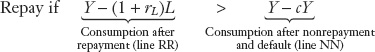
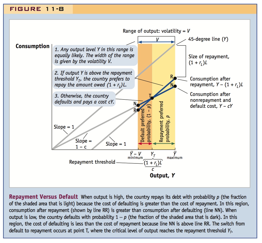
Figure 11-8 plots both sides of this inequality against Y for the case in which both repayment and default will occur within the range of possible output levels between maximum output and minimum output − V. At some critical level of output, called the repayment threshold, the government will switch from repayment to default. At this critical level, the two sides of the preceding inequality have to be equal; that is, the debt payoff amount (1 + rL)L must equal the punishment cost cY.
478
By rearranging the preceding inequality, we can find the level of Y at the repayment threshold YT and can restate the government’s choice as
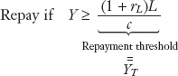
For the case shown in Figure 11-8, we assume that this repayment threshold, YT = (1 + rL)L/c, is within the range of possible outputs between the minimum − V and the maximum .
The value of consumption after repayment, Y − (1 + rL)L, is shown by the repayment line RR, which has a slope of 1: every extra $1 of output goes toward consumption, net of debt repayments. The value of consumption after nonrepayment and default, Y − cY, is shown by the nonrepayment line NN, which has a slope of (1 − c), which is less than 1: when a country has decided to default, from every extra $1 of output gained by not repaying the country’s debts, only $(1 − c) goes toward consumption, allowing for the net punishment cost.
The lines RR and NN intersect at the critical point T, and the corresponding level of output YT is the repayment threshold. Given that the slope of NN is less than the slope of RR, we can see that the country will choose to repay when output is above the repayment threshold YT (i.e., to the right of T) and to default when output is below the repayment threshold YT (i.e., to the left of T).
479
This geometric argument should be intuitively appealing. Say that p is the endogenous variable we are trying to explain, and that we will see how it responds to two exogenous changes: a change in L, and an increase in output volatility (captured by stretching the bounds of the uniform distribution).
Note that the size of the repayment region relative to the default region tells us how likely repayment is to occur relative to default. Let the probability of repayment be p. The key piece of the puzzle is to figure out what determines p. We now show how it depends on two factors: how volatile output is and how burdensome the debt repayment is.
An Increase in the Debt Burden The first variation on the model in Figure 11-8 that we consider is an exogenous increase in the level of debt payments, which we suppose increase from the original level (1 + rL)L to a new higher level  . This increase could be due to a change in the debt level, a change in the lending rate, or some combination of the two. This case is shown in Figure 11-9.
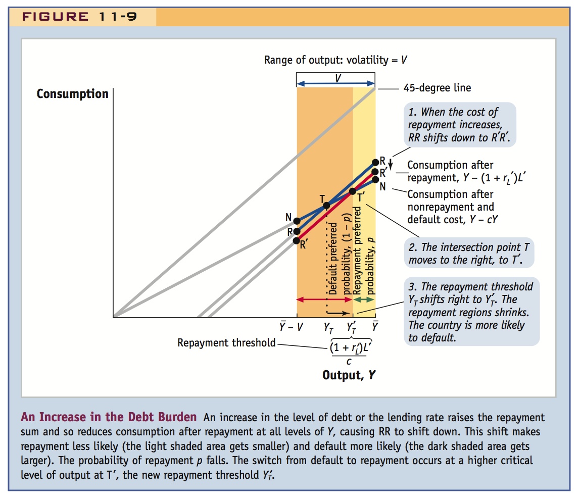
The value of consumption after repayment, Y − (1 + rL)L, must fall as (1 + rL)L rises, so line RR will shift down to R′R′. The costs of repayment are higher, and the country will find it beneficial to default more often. We can see this in the figure because after the RR curve shifts down, a greater part of the line NN will now sit above the line R′R′, and the new critical intersection point T will move to the right at T′, corresponding to the new higher repayment threshold, 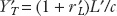 .
.
What does this mean for the probability of repayment? It must fall. The repayment region on the right is now smaller, and the default region on the left is larger. With all output levels in the two regions equally likely, the probability p that output is in the repayment region must now be lower.
480
State the conclusion: p is 1 when L is small enough, but then drops with L until it reaches 0.
We have considered only a small change in the debt burden, so the repayment region hasn’t vanished. But if the debt burden increases sufficiently, RR will shift down so far that the critical point T will shift all the way to the right, to the maximum level of output, the repayment region will disappear, and the probability of repayment will be zero (or 0%). If the debt burden is high enough, the country is always better off taking the punishment.
Conversely, if the debt burden decreases sufficiently, RR will shift up so far that the critical point T will shift all the way to the left, to the minimum level of output, the default region will disappear, and the probability of repayment will be 1 (or 100%). If the debt burden is low enough, the country will always repay.
Thus, the outcome shown in Figure 11-8 applies only when the debt burden is at some intermediate level such that the repayment threshold is between the minimum and maximum levels of output.
An Increase in Volatility of Output The second variation on the model in Figure 11-8 that we consider is an increase in the volatility of output, which we suppose increases from its original level V to a new higher level V′. This case is shown in Figure 11-10. There could be many reasons why a country is subject to higher output volatility: weather shocks to agricultural output, political instability, fluctuations in the prices of its exports, and so on.
481
Draw the graph, and note that that it is only the lower bound that is being stretched--so more bad things can happen.
In this case, the consumption levels after repayment on line RR and after default on line NN are unchanged because the debt burden is unchanged. What has changed is that there is now a much wider range of possible output levels. Higher volatility V means that output can now fall to an even lower minimum level, − V′, but can only attain the same maximum .
State this comparative static result.
Thus, an increase in V makes default more likely. In Figure 11-8, the country wanted to default whenever output fell below the critical level T, so it will certainly want to default in the wider range of low outputs brought into play by higher volatility. The default region gets larger and now includes all these new possible levels of output to the left of T. Conversely, the range of outputs to the right of T where repayment occurs is unchanged because the repayment threshold, YT = (1 + rL)L/c, is unaffected by a change in V. Hence, the probability p that output is in the repayment region must fall because the repayment region is now smaller relative to the default region.
To sum up, a rise in volatility lowers the level of debt L at which default becomes a possibility and after that point makes default more likely at any given level of L, up to the point at which default occurs with probability 100%.
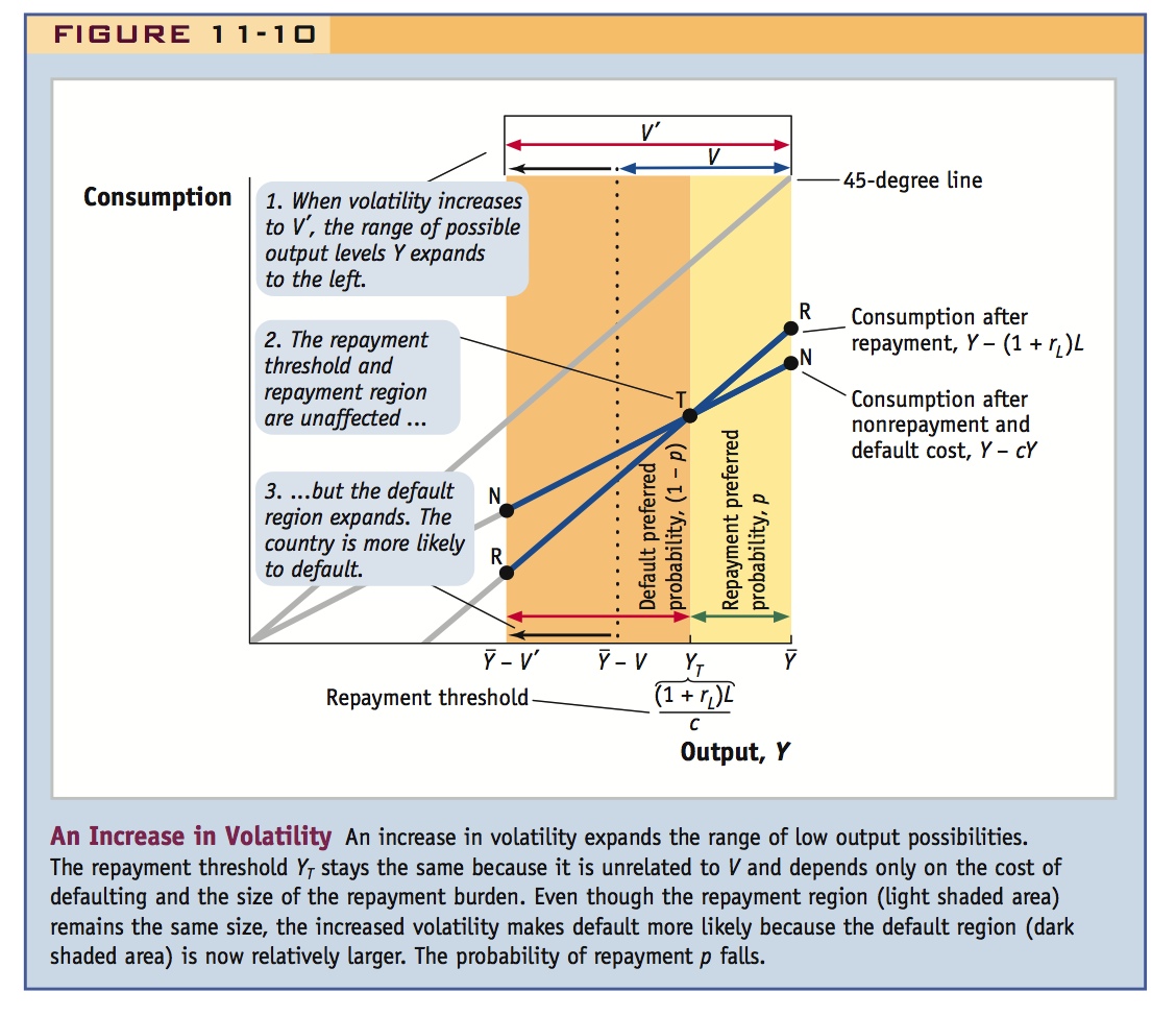
The Lender Chooses the Lending Rate All of the preceding results assume a given interest rate on the loan. But now that we know how the likely probability of repayment p is determined, we can calculate the interest rate that a competitive lender must charge. Competition will mean that lenders can only just break even and make zero expected profit. Thus, the lender will set its lending rate so that the expected revenues from each dollar lent, given by the probability of repayment p times the amount repaid (1 + rL), equal the lender’s cost for each dollar lent, which is given by (1 + r), the principal plus the risk-free interest rate at which the lender can obtain funds.
To reinforce this point, solve explicitly for the lender's return as 1 + rL = (1+r)/p.
What do we learn from this expression? The right-hand side is a constant, determined by the world risk-free rate of interest r. Thus, the left-hand side must be constant, too. If p were 1 (100% probability of repayment), the solution would be straightforward: with no risk of default and competitive lenders, the borrower will rightly obtain a lending rate equal to the risk-free rate r. But as the probability of repayment p falls, to keep the left-hand side constant, the lenders must raise the lending rate rL. That is, to compensate for the default risk, the lenders charge a risk premium so that they still just break even.
Empirical evidence that the ex post rate of return
on emerging market bonds is not much bigger than that on U.S. government bonds. Most of the risk premia were lost to defaults.
3. A Model of Default, Part Two: Loan Supply and Demand
a. Loan Supply
At low levels of debt, the probability of default is zero, so lenders charge the risk-free rate r. As debt increases, however, at debt Lv the probability of default starts to increase, so the lender charges a risk premium. The premium then increases with size of the debt (and tends to infinity as the probability of default approaches 1 at LMAX).
b. Loan Demand
Assume demand is decreasing in rL. Equilibrium occurs at a debt between Lv and LMAX
c. An Increase in Volatility
An increase in means default can occur at a lower level of debt and the probability of default increases thereafter. Supply shifts up and back because the lenders require higher premia. At the same time, borrowers want to take out more loans as a way of smoothing consumption in the face of the higher volatility, so loan demand increases. Conclusion: loan rates and the probability of default increase; if supply shifts back more than demand—as is likely for developing countries—loans decrease.
Is There Profit in Lending to Developing Countries?
Our break-even assumption may seem a little odd. A popular belief is that rich country creditors, like loan sharks, are making huge profits from lending to developing countries. But the long-run empirical evidence suggests otherwise.
Economists Christoph Klingen, Beatrice Weder, and Jeromin Zettelmeyer looked at how lenders fared in emerging markets from the 1970s to the 2000s by computing the returns on government debt in 22 borrower countries.24 They did not look at the ex ante returns that consisted of the promised repayments in the original loan contracts. Instead, they looked at the ex post returns, the realized rates of interest actually paid on the loans, allowing for any defaults, suspensions of payments, reschedulings, or other deviations from the contractual terms.
482
The results were striking, as shown by Figure 11-11. The average returns on emerging market bonds in this period were 9.1% per year. This was barely above the three-year U.S. government bond returns of 8.6% over the same period and below returns on 10-year U.S. government bonds (9.2%) and U.S. corporate bonds (10.5%). This is not because the borrowers were charged low interest rates beforehand. They were charged typical risk premiums. But if the loans had been paid off according to those terms, we would have expected that lenders would have reaped much larger returns ex post. For example, based on the typical risk premiums seen in emerging markets in the period 1998 to 2007, an extra 2.8% return would have been demanded as a risk premium ex ante, pushing ex post returns up to around 12% to 13%. But such high ex post returns were not seen, as Figure 11-11 shows: defaults ate up the risk premiums and the lenders barely broke even.
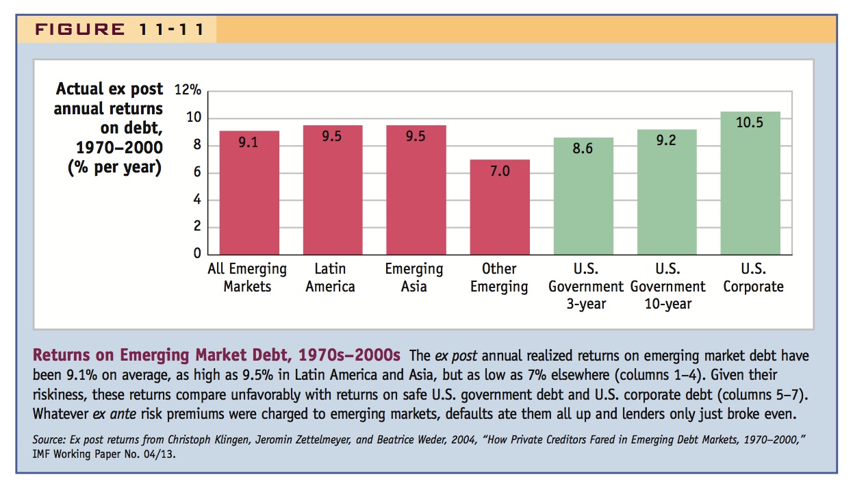
Considering the highly risky nature of emerging market debt, as compared with U.S. corporate debt, this finding is remarkable and it suggests that the break-even assumption of our simple model is not far wrong. Admittedly, there were periods when emerging market bonds paid off handsomely. In the early 1990s there were few defaults and lenders were repaid at high interest rates. But there were also periods with massive defaults, like the early 1980s, in which repeated postponements and restructurings meant that creditors got back only pennies on each dollar they had lent to the defaulting countries. Defaults are rare but cataclysmic events for creditors, so only a long-run sample can be informative. But judging from the data in Figure 11-11, lenders to emerging markets have only just broken even, if that.
This is quite interesting, and should be emphasized.
483
A Model of Default, Part Two: Loan Supply and Demand
The first steps we took in constructing the model were to understand the problem from the lender’s standpoint. Knowing the probability p that borrowers will default when output is low, lenders adjust the lending rate rL they charge depending on the volatility of output V and the level of debt L. Knowing the lending rate and the debt amount determines the loan supply curve for a country, which, combined with an understanding of loan demand, will allow us to determine equilibrium in the loan market.
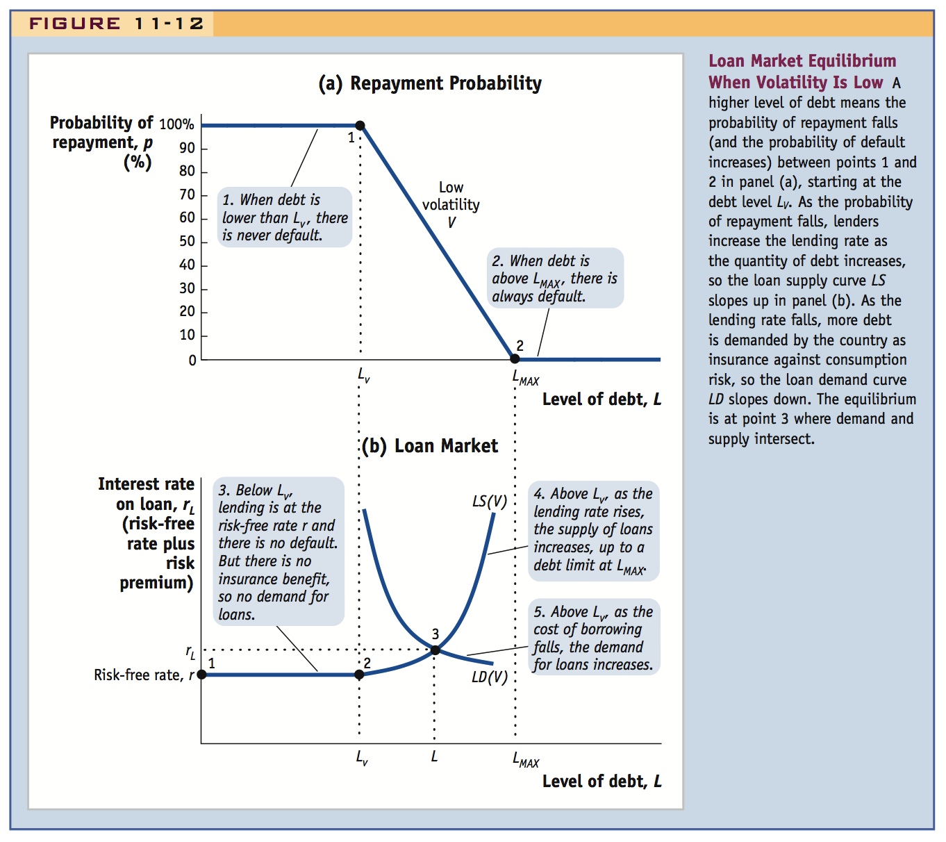
Loan Supply Suppose output volatility is at some low level V. The probability of repayment is shown in Figure 11-12, panel (a). The loan supply curve LS(V) is shown in panel (b).
This follows directly from the previous results about the effects of L on p and the determination of rL. Suggest going directly from that material--while it is fresh in students' minds--to here. Then come back and do the previous application, so it doesn't interrupt the flow of the argument.
At low levels of debt, as we saw, the probability of repayment is 100%, so a loan of size L in this range will be made at a lending rate rL that equals the risk-free rate. In this debt range, the loan supply curve is flat between points 1 and 2. Then, as debt rises above some loan size LV that depends on the volatility of the borrowing country’s output, the probability of repayment starts to fall below 1 (100%), and the break-even condition tells us that lenders will have to start increasing the lending rate so they don’t lose their shirts. At point 2 (the point at which the probability of repayment falls below 100%), the supply curve starts to slope up. For any given increase in loan size L, lenders must decide how much to increase the lending rate rL to ensure that the break-even condition is met. In making this decision, the lenders must take into account that any increases in L and/or rL will adversely affect the repayment probability p (as we saw earlier). Finally, as the loan size approaches its maximum LMAX, the rising repayment burden (higher L and higher rL) will cause the probability of repayment to approach zero. The lending rate will have to approach infinity to ensure that the loan will break even, so the loan supply curve becomes vertical as the debt limit LMAX is reached. No loans are supplied above this level of debt.
Loan Demand The equilibrium market outcome must be somewhere on the lender’s loan supply curve. But it must also be on the borrower’s loan demand curve. How is that determined? The formal derivation of borrowing demand depends on the country’s consumption preferences, including its aversion to risk; this is mathematically complex, but we can sum up the results intuitively by drawing a loan demand curve LD(V) that depends on two factors: the lending rate charged, rL, and the volatility of output, V. We restrict our attention to the normal case in which the demand curve slopes down so that an increase in the interest cost of the loan (a rise in rL) causes a decrease in the size of loan demanded (a fall in L).
We can now finish our graphical representation of the loan market equilibrium, and in Figure 11-12, panel (b), equilibrium is at point 3, where loan supply LS and loan demand LD intersect. Note that this intersection will be, as shown, between LV and LMAX. Why? Below debt level LV, the country never defaults and so debt provides no consumption-smoothing insurance in this range, and the country will want to borrow more and move up and to the right along the loan supply curve. As the cost of borrowing rises, however, the country must consider the trade-off between the amount of insurance it obtains from the debt and the rising cost of that insurance. At some point, this trade-off evens out and we reach the loan quantity the country desires. In Figure 11-12 the quantity of loans supplied and demanded will be equal at equilibrium point 3 with debt level L and lending rate rL.
484
Always ask the students to keep track of what is endogenous (L, rL, and implicitly p) and exogenous (here, volatility). The comparative static exercise we are about to undertake is then to predict how an increase in volatility affects L, rL, and p.
An Increase in Volatility What happens if the country has a higher level of volatility V′? We now show how the loan supply and demand curves will shift to LS(V′) and LD(V′), as shown in Figure 11-13.
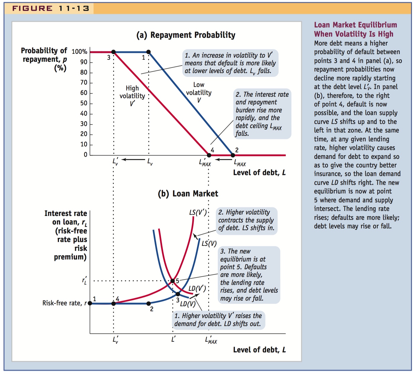
In panel (a), higher volatility means that default starts to become a possibility at a low level of debt compared with the low volatility case, as we saw previously. Once above that level of debt, repayment is less likely than when volatility is low. This means that the lending rate rises more quickly to ensure the lenders break even, and the probability of repayment reaches zero at a lower level of debt. The debt ceiling falls to a lower level  , because higher interest rates mean that the repayment burden will rise more quickly in this case as debt increases.
485
Consequently, in panel (b), the interest rate is higher at every debt level, and debt hits a ceiling at a lower level of debt. That is, we have shown that the loan supply curve shifts left and up. The lending rate starts to rise at point 4, at a lower debt level  , because higher volatility can lead to the possibility of defaults at lower levels of debt. Second, at higher debt levels, higher volatility always means a higher probability of default, so higher interest rates are imposed by lenders, all the way up to the ceiling at
  .
.
What about loan demand? When volatility rises, the loan demand curve also shifts. With typical preferences (which include risk aversion), higher volatility means that the country will want more insurance, or more consumption smoothing, all else equal. In this model, defaultable debt is the only form of insurance a country can get, so, at any given lending rate, it will want to have more debt. The loan demand curve shifts right to LD(V′).
486
State the solution to the comparative static problem.
The net result of the shifts in loan supply and demand is a new equilibrium at point 5. If loan supply moves left/up and loan demand moves right, the lending rate will definitely increase. The net effect on the amount of debt is ambiguous, however, and depends on whether the demand shift is larger than the supply shift. If the supply effect dominates, the country will end up with less debt, higher-risk premiums, and more frequent defaults—the very characteristics we see in emerging markets as compared with advanced countries.
What are the costs of default? How big are they?
a. Financial Market Penalties
Three sorts of penalties: (1) Exclusion from credit markets, usually for three to four years. (2) A downgrade in credit ratings, raising risk premia. (3) Inability to borrow in the domestic currency.
b. Broader Macroeconomic Costs and the Risk of Banking and Exchange Rate Crises
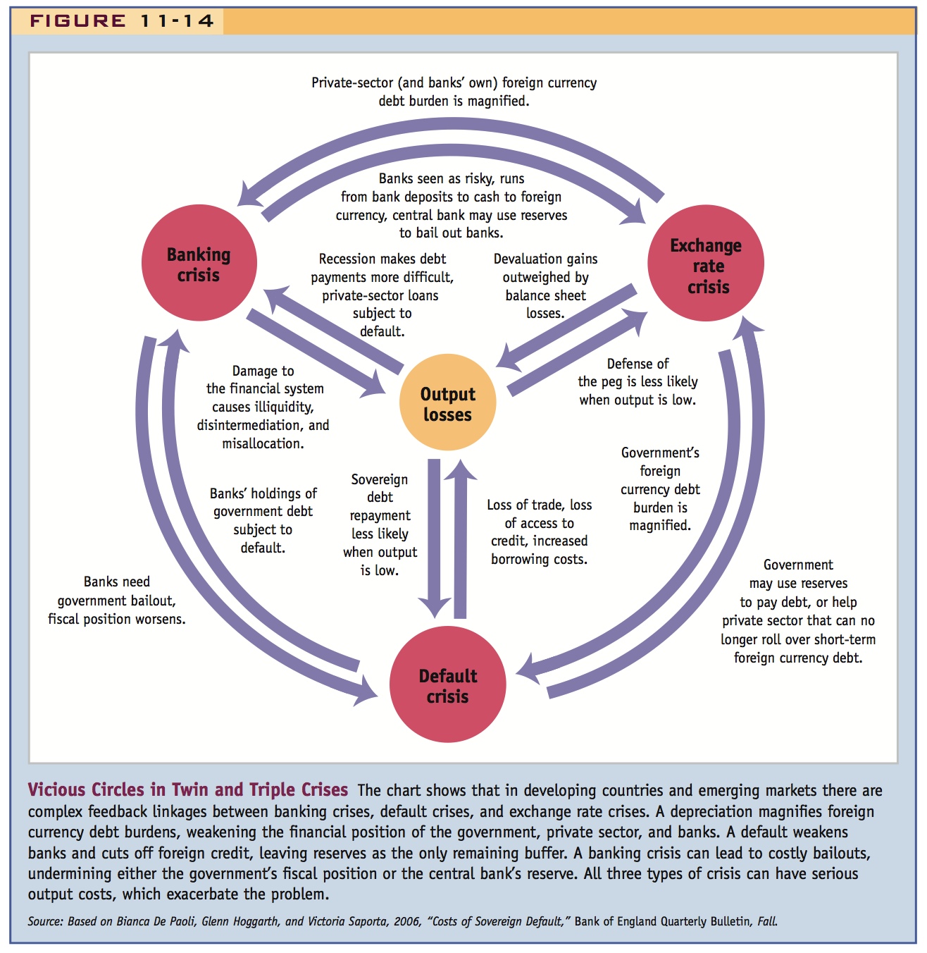
Default hurts banks because they often hold a lot of government debt. They will ask for bailouts, which stresses the government even more. Default could start a banking crisis. This could reduce lending and lead to recession. The increase in risk premia could also precipitate a currency crisis under fixed rates. So there is the potential for a vicious circle default, banking, and currency crises along with recession.
4. Conclusion
This section developed a simple model of sovereign default. It suggests that volatility is a root cause of defaults, and volatility is greater in developing countries than it developed. But some questions: (1) What causes volatility? Exogenous shocks, or poor institutions? (2) Why do developed countries have fewer defaults? The costs must be higher, greater cost of financial trauma, greater political costs in democracies.
This is a nice way of linking this material to the chapter on fixed/flexible rates: Developing countries with sovereign debt problems may be forced to borrow in foreign currency, and so are subject to adverse wealth shocks due to exchange rate fluctuations.
Similarly, this links this material to the chapter of currency and banking crises and their associated macroeconomic consequences..
The Costs of Default
Our model of default, like many others, relies on punishment costs to give debtors an incentive to repay. Is this realistic? How big are the costs? Defaulters do not get away scot-free, and to see why, we consider evidence from a Bank of England study and other research.25
Financial Market Penalties First, defaulters are excluded from further borrowing until the default is resolved though negotiations with the creditors. These exclusion periods may vary. The Bank of England study found that in the 1980s defaulters were denied market access for an average of four and a half years; however, in the easy credit atmosphere of the 1990s and 2000s, that figure dropped to an average of three and a half months. Exclusion from credit markets can create future consumption costs when the cushion of borrowing is no longer there to smooth consumption. Exclusion may impair investment, too.
Second, default is associated with a significant downgrade in credit ratings and corresponding increases in risk premiums.26 The Bank of England study found that 7 of 8 nondefaulters had credit ratings of BBB+ or better (the exception was India), but 12 of 13 past defaulters were ranked BB+ or worse (the one exception was Chile). These results applied to countries with a variety of income per capita and debt-to-GDP levels. This kind of penalty has a long history: in the first wave of globalization before 1914, defaulters on average paid an extra 1% per year in interest rate risk premiums, controlling for other factors.27
Finally, defaulters may face another major inconvenience when borrowing: an inability to borrow in their own currency. The Bank of England study found that non-defaulting countries, including India, China, Korea, Czech Republic, Malaysia, and Hungary, were able to issue between 70 and 100% of their debt in domestic currency; in contrast, a group of past defaulters, including Brazil, Mexico, Philippines, Chile, and Venezuela, only issued between 40 and 70% of their debt in their own currency. In studying fixed and floating regimes, we learned that the disadvantage of liability dollarization is that depreciations increase the costs of debt principal and interest in domestic currency terms. These changes can lead to destabilizing wealth effects because these impacts amplify debt burdens on the balance sheets of households, firms, and governments.
487
Broader Macroeconomic Costs and the Risk of Banking and Exchange Rate Crises The financial penalties are not the only cost that would-be defaulters must weigh. Default may trigger additional output costs, including the serious threats of twin or triple crises.
A default can do extensive damage to the domestic financial system because domestic banks typically hold a great deal of government debt—and they may have been coerced to hold even more such debt in the period right before a default.28 The banks will likely call for help, putting further fiscal strain on the government. But the government usually has no resources to bail out the banks at a time like this (often, it has been trying to persuade the banks to help out the government). A default crisis can then easily spawn a banking crisis. At best, if the banks survive, prudent management requires the banks to contract domestic lending to rebuild their capital and reduce their risk exposure. At worst, the banks fail. The disappearance of their financial intermediation services will then impair investment activity, and negative wealth effects will squeeze the consumption demand of depositors who lose their access to their money, temporarily or permanently, in a bank that is closed or restructured. The result is lower demand and lower output in the short run and hence more risk for banks because debtors find it harder to pay back their bank loans in recessions. Financial disruption to the real economy also disrupts a nation’s international trade. Default can disrupt the short-term credit (provided by domestic and foreign lenders) that is used to finance international trade, and there is some evidence that large and persistent trade contractions follow a default.29
In addition to a banking crisis, a default can trigger an exchange rate crisis if the country (like many emerging markets) is trying to preserve a fixed exchange rate. An increase in risk premiums on long-term loans to the government may be matched by a similar increase in risk premiums on bank deposits, especially if a banking crisis is feared. A risk premium shock of this sort, as we learned when we studied exchange rate crises, contracts money demand and causes a drain of foreign exchange reserves at the central bank as the peg is defended. At the same time, if the pleading of banks for fiscal help is ignored, the central bank will be under pressure to do a sterilized sale of reserves to allow it to act as a lender of last resort and expand domestic credit. But such activity will cause reserve levels to fall even further. The reserve drain may be large enough to break the peg, or at least damage the peg’s credibility. Expected depreciation will then enlarge the risk premium further, compounding the reserve drain. In the meantime, interest rate increases further dampen investment in the home economy, lowering output and making it harder for debts to be serviced, which hurts the banks again, lowers output again, and compounds all of the problems just outlined.
Lower output and higher-risk premiums can be expected during a default crisis, but they can also trigger banking and exchange rate crises. Low output and high-interest rates can break a contingent commitment to a peg; as we have seen in this chapter, they can generate a greater incentive to default; and we also know they can only worsen domestic financial conditions by making it harder for everyone to service their debt to banks and by damaging bank balance sheets.
488
From all these circuitous descriptions, presented schematically in Figure 11-14, the potential for a “vicious circle” of interactions should now be clear, explaining why so often the three types of crisis are observed together.
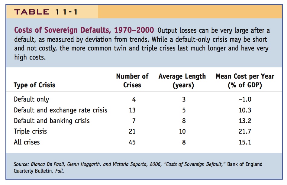
The consequences of default are therefore not pleasant. As Table 11-1 shows, when default crises occur on their own, there appear to be no costs; unfortunately, that applies in only 4 of 45 cases, less than 10% of all defaults in the sample. In every other case, there is either a twin default/exchange rate crisis (13 cases), a twin default/banking crisis (7 cases), or a triple default/exchange rate/banking crisis (21 cases). In all these other cases (more than 90% of defaults), the output losses associated with the crisis are significant, measured by deviation from trend output growth: on average, around 15% of GDP per year for eight years. That is a large cost, even if comparisons with normal trends may be misleading, because it is difficult to estimate the costs that the countries would have faced had they not defaulted.30
489
To sum up, if financial penalties and legal action provide insufficient motives for repayment, there is reason to believe that many other costs of default exist that provide enough incentive for contingent debt repayment.
Spend some time talking through this figure, since it integrates material from several previous chapters.
Important
Conclusion
We have developed a simple model in which sovereign debt is a contingent claim that will not be paid in hard times. In equilibrium borrowers obtain consumption-smoothing via debt (a form of insurance against volatile consumption levels) at a price—the risk premium—that compensates lenders for default risk. The model is too simple to capture all aspects of the default problem, such as the tendency of borrowing to move in volatile cycles, and the scope for contagion and “animal spirits” in this asset market as in any other.
Nonetheless, the model provides valuable insights and leads us to deeper questions. For example, the model assumes that output volatility is the root cause of default, and we know that output volatility is high in poorer countries. But what is behind that? In some developing countries, it could be a result of commodity specialization, terms-of-trade shocks, climate, and other economic disturbances. Yet an alternative explanation might be the poor institutional framework in these countries, which is correlated with both low incomes and high volatility. Thus, the default problem may be, deep down, a reflection of poor institutions. Poor institutions may also be generating default at lower debt levels through nonvolatility channels: they may obscure financial transparency, generate weak property rights, prevent credit monitoring, encourage corruption and bribery, allow for the misuse of loans, lead politicians to focus on the short term (with risky overborrowing), and so on—all of which add to the risk premium, all else equal.
490
How did advanced countries eventually find a way to avoid these outcomes? Our model suggests that all countries want to default at some debt level, but for advanced countries, that level might be very high. Why? The model says it must be that the costs of default in such countries are much higher. There may be truth to this on two dimensions: economic and political. Economically, a sovereign default in an advanced country would wreck a highly developed financial system, whereas in poorer countries the very lack of financial sophistication probably keeps such costs lower. In addition, the political costs are higher in advanced countries, in that a large, democratically empowered, and wealth-holding middle class is likely to punish governments that take such actions; in poorer countries, the political costs may be smaller if the losers are fewer or political accountability is weaker.
Every few years, in a tranquil time, some expert predicts that there will not be any more sovereign defaults. They can’t be taken very seriously. History does suggest that many of the deep and intertwined underlying political-economy problems can be solved, but it may take an awfully long time for countries to overcome these impediments and emerge from the serial default club.31
A case study of intertwined default, banking, and exchange rate crises.
The perfect example of a triple crisis.
The Argentina Crisis of 2001–2002
In this section we focused on the problem of default. But we also emphasized (as in Figure 11-14) the feedback mechanisms at work in twin and triple crisis situations in which default crises, exchange rate crises, and banking crises may simultaneously occur. Just as in the case of self-fulfilling exchange rate crises (explained in the chapter on crises), these “vicious circles” may lead to self-fulfilling twin and triple crises where, as the economist Guillermo Calvo puts it, “If investors deem you unworthy, no funds will be forthcoming and, thus, unworthy you will be.” In general, theory and empirical work suggest that bad fundamentals only make the problem of self-fulfilling crises worse, and disentangling the two causes can be difficult, leading to ongoing controversy over who or what is to blame for any given crisis. The Argentina crisis of 2001–02 dramatically illustrates these problems.32
Background Argentina successfully ended a hyperinflation in 1991 with the adoption of a rigidly fixed exchange rate system called the Convertibility Plan, and a 1-to-1 peg of the peso to the U.S. dollar. As we noted in a previous chapter, this system operated with high reserve backing ratios and (in theory) strict limits on central bank use of sterilization policy. The Convertibility Plan was a quasi currency board.
491
With a firm nominal anchor, Argentina’s economy grew rapidly up to 1998, apart from a brief slowdown after the Mexican (Tequila) crisis in 1994. The country was able to borrow large amounts at low-interest rates in the global capital market. The only troubling sign at this point was that despite boom conditions the government ran persistent deficits every year, increasing the public debt to GDP ratio. Most of this debt was held by foreigners, which increased Argentina’s net external debt relative to GDP. Given the long-run budget constraints (for the government, and for the country) these deficits were unsustainable.
In 1997 crises in Asia were followed by increases in emerging market risk premiums, and these shocks were magnified by crises in 1998 in Russia and Brazil. The Brazil crisis also led to a slowdown and depreciation in one of Argentina’s major trading partners. At the same time, the U.S. dollar started to appreciate, dragging the Argentina peso into a stronger position against all currencies. Higher interest rates, lower demand abroad, and an appreciated exchange rate put the Argentine economy into a recession.
Dive With these changes in external conditions, Argentina’s macroeconomic regime started to unravel. The recession worsened an already bad fiscal situation. Because no surpluses had been run in the good times, there was no cushion in the government accounts, and the red ink grew. Public debt, which had been 41% of GDP in 1998, grew to 64% of GDP in 2001. Foreign creditors began to view these debt dynamics as possibly explosive and inconsistent with the long-run budget constraint, implying a risk of default. The creditors demanded higher interest rates for new loans and refinancings, which only increased the rate of debt explosion. Risk premiums on long-term government debt blew up, from 3% to 4% in late 1997 to 7% to 8% in late 2000.
The fiscal situation thus damaged the economy and the banking sector, as higher interest rates depressed aggregate demand in the short run, and caused a deterioration of banks’ balance sheets (as loans went bad and other assets declined in value). This deterioration, in turn, made the fiscal situation worse, because in a recession tax revenues tend to fall and government social expenditures tend to rise. The government needed to borrow more, even as the lenders started to withdraw.
In addition, the situation posed a threat to the monetary regime and the Convertibility Plan. People were worried that if the government accounts worsened further, then all public credit would be turned off, and if the government were then unwilling to impose the austerity of spending cuts in mid-recession, it would have had to finance the deficit using the inflation tax. Finally, even if the government did not use inflationary finance, it still might want to use temporary monetary policy autonomy to relieve the recession through a devaluation and lower interest rates, both of which would make the peg not credible. Either or both of these threats would expose the peg to the risk of a speculative attack.
In addition, people knew that if the banks got into trouble, they would need to call on the central bank to act as a lender of last resort, as they had in 1994 (when reserves had plummeted and a crisis was averted only by a last-minute lifeline from the International Monetary Fund [IMF]). If people felt that their deposits would be safer in Miami or Montevideo, there would be a massive run from deposits to peso cash to dollars, overwhelming even the substantial foreign exchange reserves at the central bank.
492
Crash In 2001 all of these forces gathered in a perfect storm. Politically, fiscal compromise proved impossible between the two main political forces (the weak President Fernando de la Rúa of the Radical Party and the powerful Peronist provincial governors). The provinces collected and spent large amounts of national tax revenue and were not willing to make sacrifices to help de la Rúa, a political opponent. They gambled, correctly, that a crisis would bring them to power (even at the cost of destroying the country).
By mid-2001, private creditors had almost walked away from Argentina and the last-gasp effort involved a swap of short-term high interest rate debt for long-term very high interest rate debt, with an annual yield near 15%. Markets were unimpressed—this scheme bought a few months of breathing space on principal payments, but left Argentina with an even worse debt service problem down the road. Private lending dried up and despite a (noncredible) announcement of a zero deficit rule in July, the risk premium on government debt exploded, from 10% in June to 15% in August, and approached 20% in October. As the debt burden grew and the economy sank, we know from this chapter that default would be increasingly likely.
There was only one lender left now, the IMF. But they were increasingly as unimpressed with Argentina’s policy shenanigans as everyone else. In a move that it doubted at the time and regretted soon thereafter, the IMF made one last big loan to Argentina in August 2001. The money was poured into the government’s coffers and into the Central Bank’s dwindling pot of reserves, but it didn’t last very long.
The banks were in a very weak state. Economic conditions were raising the number of nonperforming loans anyway. But banks had also been coerced or persuaded that it would be a good idea for them to buy large amounts of the government’s debt in 2001. This dollar debt carried a high interest rate, but was also risky, because of the possibility of default and/or exchange rate depreciation after a crisis. Depositors knew this and they also knew that banks would probably fail if the central bank and the government could not protect them.
The End The three crises were all now shaping up to happen, encouraged by output contractions, consistent with the “vicious circle” dynamics shown in Figure 11-14. The final act came in November. The IMF concluded that the economy was not being turned around by any of the policies in place and that further loans were therefore a waste of time unless Argentina made radical adjustments, including considering the possibilities of devaluing, defaulting, and even dollarizing. The government would have none of it, and when the IMF announced no more credit, the public knew the game was up, and seeking to put their assets in a safe haven, they started a massive run on the banks. To stem the flow, the government imposed capital controls (corralito) to stop such activity, and also froze the majority of bank deposits.
This triggered a political explosion, violence and unrest, and within days de la Rúa was history, airlifted from the Casa Rosada by helicopter. His numerous successors over the following weeks initiated a default on the public debt (the world’s biggest-ever default at the time) and allowed the exchange rate to float (it fell to 4 pesos to the dollar very quickly). The private sector was awash with unserviceable dollar liabilities, so the government “pesified” them, causing utter chaos in the courts and grave economic uncertainty. The banks were barely functional for several months, and the savings of many Argentines vanished. Taxes were raised and government spending cut. The economy went from a bad recession to total meltdown, amid scenes of previously unimaginable poverty and deprivation.
493
Argentina’s policies were inconsistent. When the government chose a fixed exchange rate, it had to accept its pros and cons, including the risk of larger recessions when external conditions were unfavorable. But they also had to accept that a fixed exchange rate ruled out the inflation tax and placed limits on the lender of last resort capacity of a central bank faced with capital flight. Such concerns would not have been as important if the country had kept its fiscal policy in check and maintained access to credit, but in 2001 the country simply had no more room for maneuver.
Postscript As of 2007, there had been no major crisis since 2001, world economic conditions had been fairly benign, and many countries had built up large exchange reserves. This led many observers to call into question the need for the IMF, given its perceived failings in the 1997–2001 crises, and the small size of its lending capabilities in the face of growing private sector financial flows. On the other hand, international economic crises have been around for a very long time, so to more seasoned observers, it seemed a little premature for some to be calling for dismantling the only emergency service we have (see Headlines: Is the IMF “Pathetic”?). They were proved right when during and after the global financial crisis in 2008, the IMF was called to the scene of many macroeconomic accidents, including in several so-called advanced countries, to provide rescue funding.