2 Interest Rates in the Short Run: Money Market Equilibrium

The previous section laid out the essentials of the asset approach to exchange rates. Figure 4-1 sums up the uncovered interest parity relationship at the heart of the asset approach. The spot exchange rate is the output (endogenous variable) of this model, and the expected future exchange rate and the home and foreign interest rates are the inputs (exogenous variables). But where do these inputs come from? In the last chapter, we developed a theory of the long-run exchange rate, the monetary approach, which can be used to forecast the future exchange rate. That leaves us with just one unanswered question: How are current interest rates determined?

Money Market Equilibrium in the Short Run: How Nominal Interest Rates Are Determined

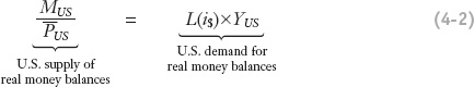
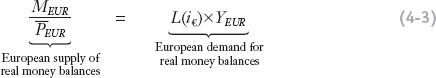
Having seen how the supply and demand for money work in the previous chapter, we can build on that foundation here. We consider two money markets in two locations: the United States and Europe. Both markets are in equilibrium with money demand equal to money supply. In both locations, the money supply is controlled by a central bank and is taken as given; the demand for real money balances M/P = L(i)Y is a function of the interest rate i and real income Y.

The Assumptions It is important to understand the key difference between the way we approach money market equilibrium in the short run (in this chapter) and the way we approached it in the long run (in the last chapter).

In the last chapter, we made the following long-run assumptions:

• In the long run, the price level P is fully flexible and adjusts to bring the money market to equilibrium.
• In the long run, the nominal interest rate i equals the world real interest rate plus domestic inflation.

In this chapter, we make short-run assumptions that are quite different:

• In the short run, the price level is sticky; it is a known predetermined variable, fixed at (the bar indicates a fixed value).
• In the short run, the nominal interest rate i is fully flexible and adjusts to bring the money market to equilibrium.

Why do we make different assumptions in the short run?

First, why assume prices are now sticky? The assumption of sticky prices, also called nominal rigidity, is common to the study of macroeconomics in the short run. Economists have many explanations for price stickiness. Nominal wages may be sticky because of long-term labor contracts. Nominal product prices may be sticky because of contracts and menu costs; that is, firms may find it costly to frequently change their output prices. Thus, although it is reasonable to assume that all prices are flexible in the long run, they may not be in the short run.

Second, why assume that interest rates are now flexible? In the previous chapter, we showed that nominal interest rates are pinned down by the Fisher effect (or real interest parity) in the long run: in that case, the home nominal interest rate was equal to the world real interest rate plus the home rate of inflation. However, recall that this result does not apply in the short run because it is derived from purchasing power parity—which, as we know, only applies in the long run. Indeed, we saw evidence that in the short run real interest rates fluctuate in ways that deviate from real interest parity.

The Model With these explanations of our short-run assumptions in hand, we can now use the same general monetary model of the previous chapter and write down expressions for money market equilibrium in the two countries as follows:

To recap: In the long run, prices adjust to clear the money market and bring money demand and money supply into line. In the short run, when prices are sticky, such adjustment is not possible. However, nominal interest rates are free to adjust. In the short run, the nominal interest rate in each country adjusts to bring money supply and money demand into equilibrium.

Money Market Equilibrium in the Short Run: Graphical Solution

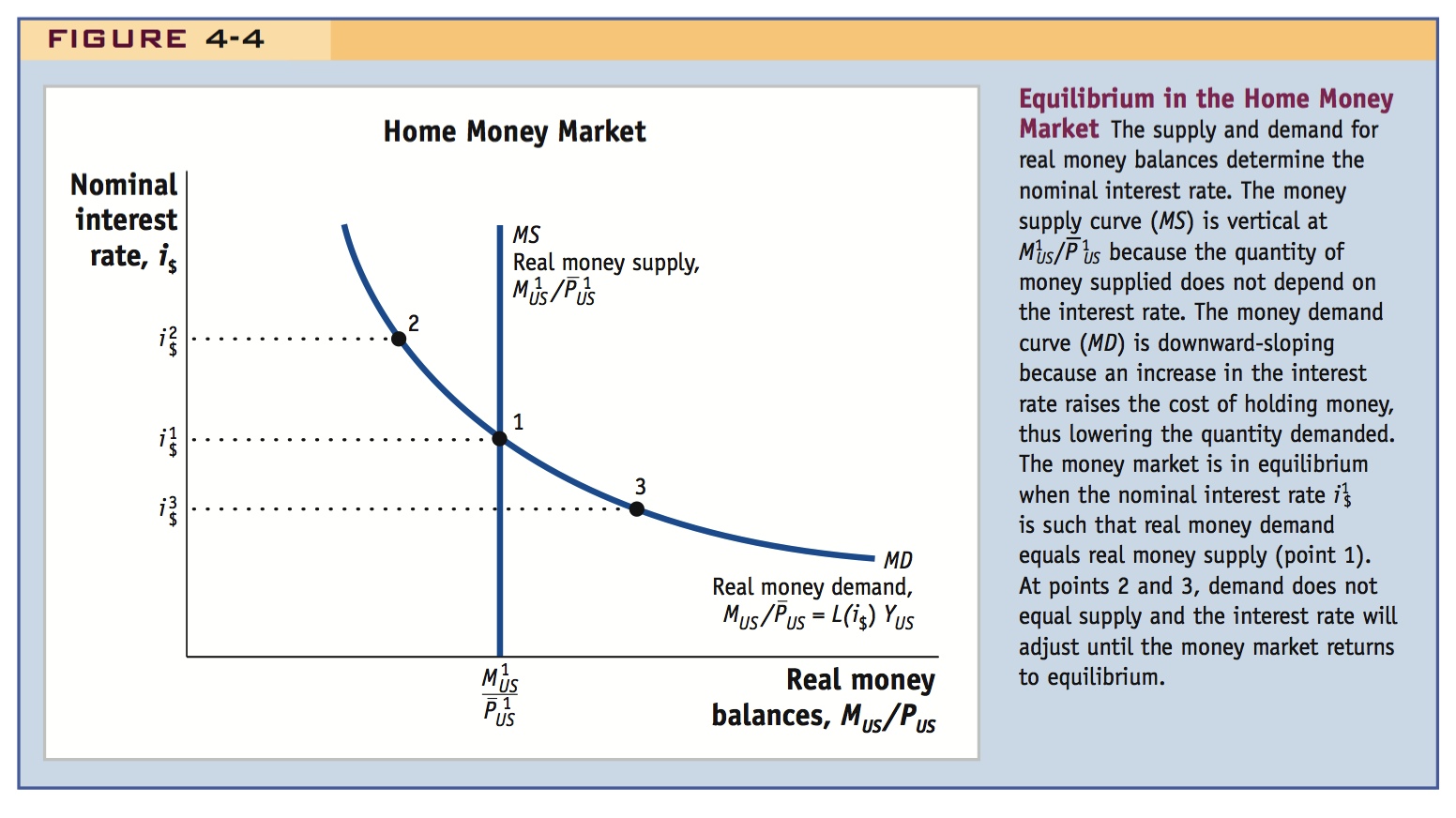
Figure 4-4 represents the U.S. money market (a similar diagram applies to the European market). On the horizontal axis is the quantity of U.S. real money balances M_US/P_US and on the vertical axis is the U.S. nominal interest rate i_$. The vertical line represents the supply of real money balances; this supply is fixed by the central bank at the level and is independent of the level of the interest rate. The downward-sloping line represents the demand for real money balances, L(i_$) × Y_US. Demand decreases as the U.S. nominal interest rate increases because the opportunity cost of holding money rises and people don’t want to hold high money balances. The money market is in equilibrium at point 1: the demand and supply of real money balances are equal at and at a nominal interest rate .

Adjustment to Money Market Equilibrium in the Short Run

If interest rates are flexible in the short run, as we assume they are, there is nothing to prevent them from adjusting to clear the money market. But how do market forces ensure that a nominal interest rate is attained? The adjustment process works as follows.

Suppose instead that the interest rate was , so that we were at point 2 on the real money demand curve. At this interest rate, real money demand is less than real money supply. In the aggregate, the central bank has put more money in the hands of the public than the public wishes to hold. The public will want to reduce its cash holdings by exchanging money for interest-bearing assets such as bonds, saving accounts, and so on. That is, they will save more and seek to lend their money to borrowers. But borrowers will not want to borrow more unless the cost of borrowing falls. So the interest rate will be driven down as eager lenders compete to attract scarce borrowers. As this happens, back in the money market, in Figure 4-4, we move from point 2 back toward equilibrium at point 1.

A similar story can be told if the money market is initially at point 3, where there is an excess demand for money. In this case, the public wishes to reduce their savings in the form of interest-bearing assets and turn them into cash. Now fewer loans are extended. The loan market will suffer an excess demand. But borrowers will not want to borrow less unless the cost of borrowing rises. So the interest rate will be driven up as eager borrowers compete to attract scarce lenders. These adjustments end only when point 1 is reached and there is no excess supply of real money balances.

Another Building Block: Short-Run Money Market Equilibrium

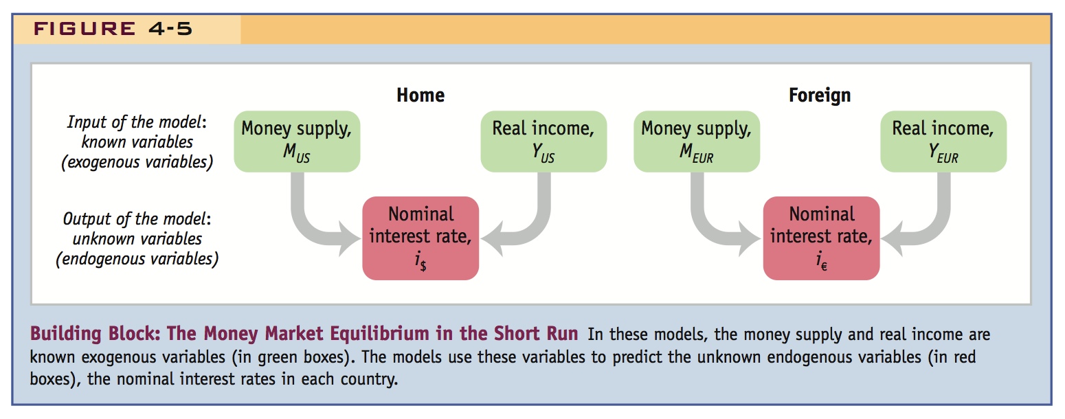
This model of the money market may be familiar from previous courses in macroeconomics. The lessons that are important for our theory of exchange rates are summed up in Figure 4-5. We treat the price level in each country as fixed and known in the short run. We also assume that the money supply and real income in each country are known. The equilibrium equations for the money market, Equations (4-2) and (4-3), then tell us the interest rates in each country. Once these are known, we can put them to use in another building block seen earlier: the interest rates can be plugged into the fundamental equation of the asset approach to exchange rate determination, Equation (4-1), along with the future expected exchange rate derived from a forecast based on the long-run monetary model of the previous chapter. In that way, the spot exchange rate can finally be determined.

Changes in Money Supply and the Nominal Interest Rate

Money market equilibrium depends on money supply and money demand. If either changes, the equilibrium will change. To help us better understand how exchange rates are determined, we need to understand how these changes occur.

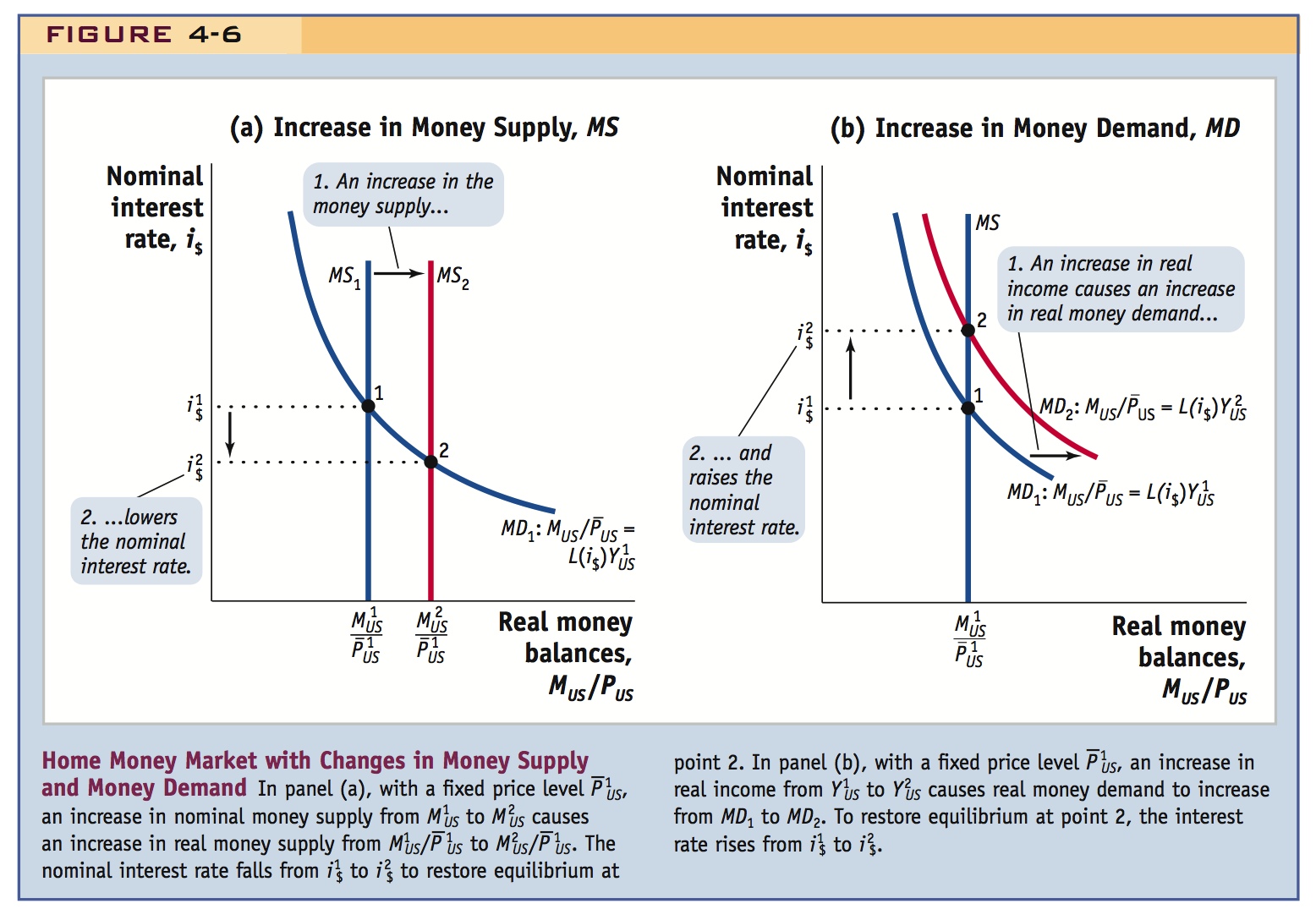
Figure 4-6, panel (a), shows how the money market responds to a monetary policy change consisting of an increase in Home (U.S.) nominal money supply from to . Because, by assumption, the U.S. price level is fixed in the short run at , the increase in nominal money supply causes an increase in real money supply from to . In the figure, the money supply curve shifts to the right from MS₁ to MS₂. Point 1 is no longer an equilibrium; at the interest rate , there is now an excess supply of real money balances. As people move their dollars into interest-bearing assets to be loaned out, the interest rate falls from to , at which point the money market is again in equilibrium at point 2. By the same logic, a reduction in the nominal money supply will raise the interest rate.

To sum up, in the short run, all else equal, an increase in a country’s money supply will lower the country’s nominal interest rate; a decrease in a country’s money supply will raise the country’s nominal interest rate.

Fortunately, our graphical analysis shows that, for a given money demand curve, setting a money supply level uniquely determines the interest rate and vice versa. Hence, for many purposes, the money supply or the interest rate may be used as a policy instrument. In practice, most central banks tend to use the interest rate as their policy instrument because the money demand curve may not be stable, and the fluctuations caused by this instability would lead to unstable interest rates if the money supply were set at a given level as the policy instrument.

Can Central Banks Always Control the Interest Rate? A Lesson from the Crisis of 2008–2009

In our analyses so far, we have assumed that central banks can control the money market interest rate, and that they can effectively do so whether they set the interest rate or the money supply. These assumptions are critical in this chapter and in the rest of this book. But are they really true? In general, perhaps, but policy operations by central banks can be undermined by financial market disruptions. Recent events in many countries illustrate the problem.

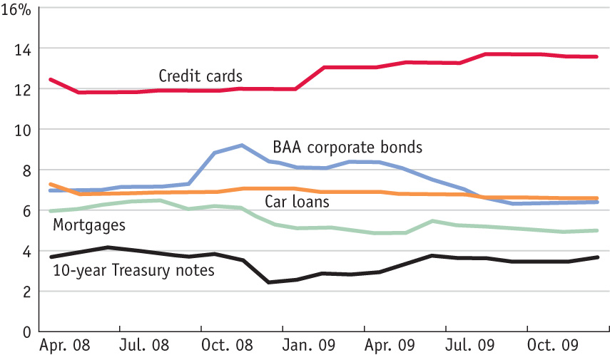
In the United States, for example, the Federal Reserve sets as its policy rate the interest rate that banks charge each other for the overnight loan of the money they hold at the Fed. In normal times, changes in this cost of short-term funds for the banks are usually passed through into the market rates the banks charge to borrowers on loans such as mortgages, corporate loans, auto loans, and so forth, as well as on interbank loans between the banks themselves. This process is one of the most basic elements in the so-called transmission mechanism through which the effects of monetary policy are eventually felt in the real economy.

In the recent crisis, however, banks regarded other banks and borrowers (and even themselves) as facing potentially catastrophic risks. As a result, they lent much less freely and when they did loan, they charged much higher interest rates to compensate themselves for the risk of the loan suffering a loss or default. Thus, although the Fed brought its policy rate all the way down from 5.25% to 0% in 2007 and 2008, there was no similar decrease in market rates. In fact, market interest rates barely moved at all, and even the credit that was available at more favorable rates was often restricted by tighter lending standards; total credit expanded very little, and refinancings were limited.

A second problem arose once policy rates hit the zero lower bound (ZLB). At that point, the central banks’ capacity to lower the policy rate further was exhausted. However, many central banks wanted to keep applying downward pressure to market rates to calm financial markets. The Fed’s response was a policy of quantitative easing.

Usually, the Fed expands base money M0 by either lending to banks which put up safe government bonds as collateral, or by buying government bonds outright in open-market operations—although these actions are taken only in support of the Fed’s interest rate target. But in the crisis, and with interest rates stuck at a floor, the Fed engaged in a number of extraordinary policy actions to push more money out more quickly:

1. It expanded the range of credit securities it would accept as collateral to include lower-grade, private-sector bonds.
2. It expanded the range of securities that it would buy outright to include private-sector credit instruments such as commercial paper and mortgage-backed securities.
3. It expanded the range of counterparties from which it would buy securities to include some nonbank institutions such as primary dealers and money market funds.

As a result of massive asset purchases along these lines, M0 in the United States more than doubled to over a trillion dollars. However, there was very little change in M1 or M2, indicating that banks had little desire to translate the cash they were receiving from the Fed into the new loans and new deposits that would expand the broad money supply.

124

Similar crisis actions were taken by the Bank of England and, eventually, by the European Central Bank (ECB); both expanded their collateral rules, although their outright purchase programs were more narrowly focused on aggressive use of open-market operations to purchase large quantities of U.K. and Eurozone government bonds (though in the ECB’s case this included low-grade bonds from crisis countries such as Greece and Portugal).

A broken transmission: the Fed’s extraordinary interventions did little to change private credit market interest rates from 2008 through 2009.

Courtesy Robert Hall/The Federal Reserve Bank of Minneapolis

To sum up, with the traditional transmission mechanism broken, central banks had to find different tools. In the Fed’s case, by directly intervening in markets for different types of private credit at different maturities, policy makers hoped to circumvent the impaired transmission mechanism. Would matters have been much worse if the central banks had done nothing at all? It’s hard to say. However, if the aim was to lower market interest rates in a meaningful way and expand broader monetary aggregates, it is not clear that these policies had significant economic effects.

Changes in Real Income and the Nominal Interest Rate

Figure 4-6, panel (b), shows how the money market responds to an increase in home (U.S.) real income from to . The increase in real income causes real money demand to increase as reflected in the shift from MD₁ to MD₂. At the initial interest rate , there is now an excess demand for real money balances. To restore equilibrium at point 2, the interest rate rises from to to encourage people to hold lower dollar balances. Similarly, a reduction in real income will lower the interest rate.

To sum up, in the short run, all else equal, an increase in a country’s real income will raise the country’s nominal interest rate; a decrease in a country’s real income will lower the country’s nominal interest rate.

The Monetary Model: The Short Run Versus the Long Run

The short-run implications of the model we have just discussed differ from the long-run implications of the monetary approach we presented in the previous chapter. It is important that we look at these differences, and understand how and why they arise.

Consider the following example: the home central bank that previously kept the money supply constant suddenly switches to an expansionary policy. In the following year, it allows the money supply to grow at a rate of 5%.

• If such annual expansions are expected to be a permanent policy in the long run, the predictions of the long-run monetary approach and Fisher effect are clear. All else equal, a five percentage point increase in the rate of home money growth causes a five percentage point increase in the rate of home inflation and a five percentage point increase in the home nominal interest rate. The home interest rate will then rise in the long run when prices are flexible.
• If this expansion is expected to be temporary, then the short-run model we have just studied in this chapter tells a very different story. All else equal, if the home money supply expands, the immediate effect is an excess supply of real money balances. The home interest rate will then fall in the short run when prices are sticky.

These different outcomes illustrate the importance of the assumptions we make about price flexibility. They also point out the importance of the nominal anchor in monetary policy formulation and the constraints that central banks have to confront. The different outcomes also explain some apparently puzzling linkages among money, interest rates, and exchange rates. In both of the previous cases, an expanded money supply leads to a weaker currency. However, in the short run, low interest rates and a weak currency go together, whereas in the long run, high interest rates and a weak currency go together.

What is the intuition for these findings? In the short run, when we study the impact of a lower interest rate and we say “all else equal,” we have assumed that expectations have not changed concerning future exchange rates (or money supply or inflation). In other words, we assume (implicitly) a temporary policy that does not tamper with the nominal anchor. In the long run, if the policy turns out to be permanent, this assumption is inappropriate; prices are flexible and money growth, inflation, and expected depreciation now all move in concert—in other words, the “all else” is no longer equal.

A good grasp of these key differences between the short- and long-run approaches is essential to understanding how exchange rates are determined. To cement our understanding, in the rest of the chapter we explore the different implications of temporary and permanent policy changes. To make our exploration a bit easier, we now lay out the short-run model in a succinct, graphical form.