4 A Complete Theory: Unifying the Monetary and Asset Approaches
Summary of the asset approach: two money-market equilibrium conditions and UIP; price levels exogenously fixed, and interest rates and the spot rate endogenous. Summary of the monetary approach: Two money-market equilibrium conditions and PPP; price levels and the exchange rate are endogenous. Assume perfect foresight.
1. Long-Run Policy Analysis
When shocks are permanent, the expected future spot rate can no longer be exogenous. To see what happens in the short run we have to solve backward from the long run in order to see how people change their expectations.
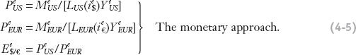
In this section, we extend our analysis from the short run to the long run, and examine permanent as well as temporary shocks. To do this, we put together a complete theory of exchange rates that couples the long-run and short-run approaches, as shown schematically in Figure 4-11:
- We need the asset approach (this chapter) — short-run money market equilibrium and uncovered interest parity:
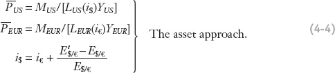
- There are three equations and three unknowns (two short-run nominal interest rates and the spot exchange rate). The future expected exchange rate must be known, as must the current levels of money and real income. (The price level is also treated as given.)
- But to forecast the future expected exchange rate, we also need the long-run monetary approach from the previous chapter—a long-run monetary model and purchasing power parity:
- There are three equations and three unknowns (two price levels and the exchange rate). Note that all variables here have a superscript e to denote future expected values or forecasts. We assume that forecasts of future money, real income, and nominal interest rates are known. This model can then be applied to obtain price forecasts and, hence, a forecast of the future expected exchange rate.2
Students will find this complicated at first: Have them list what is endogenous and exogenous. Figure 4-11 will help.
Figure 4-11 sums up all the theory we have learned so far in the past two chapters. It shows how all the pieces fit together. In total we have six equations and six unknowns.
It is only now, with all the building blocks in place, that we can fully appreciate how the two key mechanisms of expectations and arbitrage operate in a variety of ways to determine exchange rates in both the short run and the long run. Ensure you are comfortable with all of the building blocks—how they work individually and how they connect.
After all our hard work, we have arrived at a complete theory to explain exchange rates in the short run and the long run. The model incorporates all of the key economic fundamentals that affect exchange rates and, in practice, although forex markets exhibit a great deal of turbulence and uncertainty, there is evidence that these fundamentals play a major role in shaping traders’ decisions (see Side Bar: Confessions of a Forex Trader).
Long-Run Policy Analysis
When and how can we apply the complete model? The downside of working with the complete model is that we have to keep track of multiple mechanisms and variables; the upside is that the theory is fully developed and can be applied to short-run and long-run policy shocks.
The temporary shocks we saw in the last section represent only one kind of monetary policy change, one that does not affect the long-run nominal anchor. The fact that these shocks were temporary allowed us to conduct all of the analysis under the assumption that the long-run expected level of the exchange rate remained unchanged.
133
Now emphasize how a permanent change will affect both prices (over time), and expectations (now).
When the monetary authorities decide to make a permanent change, however, this assumption of unchanged expectations is no longer appropriate. Under such a change, the authorities would cause an enduring change in all nominal variables; that is, they would be electing to change their nominal anchor policy in some way. Thus, when a monetary policy shock is permanent, the long-run expectation of the level of the exchange rate has to adjust. This change will, in turn, cause the exchange rate predictions of the short-run model to differ from those made when the policy shock was only temporary.
134
Results of a survey of FX traders, revealing how they form forecasts.
a. A Permanent Shock to the Home Money Supply
b. The Long Run: A permanent increase in MU.S. must ultimately cause a proportional increase in U.S. prices (by the quantity theory) and a proportional depreciation of the dollar (by PPP). Since the real money supply doesn’t change, i$ won’t change. Since the new long-run exchange rate will be stable, people set their expectations equal to it, and the FR curve shifts up to achieve this exchange rate.
c. The Short Run: Two things happen simultaneously. First, i$ falls, since prices are sticky. This causes the DR curve to shift down, so that the dollar tends to depreciate. Second, people expect the future depreciation of the dollar, so they buy it now: the FR curve shifts up, causing the dollar to depreciate. In the short run, the dollar will depreciate by more than it will in the long run.
d. Adjustment from Short Run to Long Run: Over time the U.S. price level increases, reducing the real money supply until returns to where it started. This causes the DR curve to shift back up until the exchange rate appreciates to achieve the new long-run exchange rate.
2. Overshooting
Given sticky prices, a permanent increase in the money supply will cause the exchange rate depreciates by more in the short run than it will in the long run. There is overshooting.
Confessions of a Foreign Exchange Trader
Trying to forecast exchange rates is a major enterprise in financial markets and serves as the basis of any trading strategy. A tour of the industry would find many firms offering forecasting services at short, medium, and long horizons. Forecasts are generally based on three methodologies (or some mix of all three):
- Economic fundamentals. Forecasts are based on ideas developed in the past two chapters. Exchange rates are determined by factors such as money, output, interest rates, and so on; hence, forecasters try to develop long- and short-range predictions of these “fundamental” variables. Example: “The exchange rate will depreciate because a looser monetary policy is expected.”
- Politics. Forecasts recognize that some factors that are not purely economic can affect exchange rates. One is the outbreak of war (see the application at the end of this chapter). Political crises might matter, too, if they affect perceptions of risk. Changes in risk interfere with simple interest parity and can move exchange rates. Making such forecasts is more qualitative and subjective, but it is still concerned with fundamental determinants in our theory. Example: “The exchange rate will depreciate because a conflict with a neighboring state raises the probability of war and inflation.”
- Technical methods. Forecasts rely on extrapolations from past behavior. Trends may be assumed to continue (“momentum”), or recent maximum and minimum values may be assumed to be binding. These trading strategies assume that financial markets exhibit some persistence and, if followed, may make such an assumption self-fulfilling for a time. Nonetheless, large crashes that return asset prices back to fundamental levels can burst such bubbles. Example: “The exchange rate has hit this level three times this year but never gone further; it will not go further this time.”
A recent survey of U.K. forex traders provided some interesting insights into this world.* One-third described their trading as “technically based,” and one-third said their trades were “fundamentals-based”; others were jobbing or trading for clients.
The survey revealed that insights from economic theory mattered little from one hour to the next. In the very short run, within the day, traders confessed that many factors unrelated to economic fundamentals affected exchange rates in the market: 29% cited “bandwagon effects,” and 33% mentioned “overreaction to news.” Concerning within-day changes in exchange rates, when asked, “Do you believe exchange rate movements accurately reflect changes in the fundamental value,” fully 97% of the traders responded no and only 3% yes. However, in the medium run, described as within six months, 58% responded yes. And in the long run, described as more than six months, 87% thought that changes reflected fundamentals.
Which economic fundamentals mattered? News about money supplies, interest rates, and GDP levels was quickly incorporated into trading, usually in less than a minute or even in a matter of seconds. All of these are key variables in our complete model. As we would expect, PPP was deemed irrelevant within the day, but 16% thought it mattered in the medium run, and 44% in the long run. The lack of unanimity about PPP may reflect legitimate concerns about its shortcomings (which we examined in the previous chapter).
* Yin-Wong Cheung, Menzie D. Chinn, and Ian W. Marsh, 2004, “How Do UK-Based Foreign Exchange Dealers Think Their Market Operates?” International Journal of Finance and Economics, 9(4), 289–306.
This is an important lesson to impart, so emphasize it before you undertake the comparative static problem: Say that since the current spot rate depends upon what people expect it to be in the future, the way to solve the model is to pin down the future and work back to the present.
These insights guide our analysis of permanent policy shocks. They also tell us that we cannot approach such analysis chronologically. Before we can figure out what happens in the short run, we have to know expectations, that is, what is going to happen in the long run. Thus, we have to use a technique that is common in forward-looking economic problems: we must solve backward from the future to the present. (This ordering mirrors the presentation of the material in this textbook—we must understand the long run before we can understand the short run.)
A Permanent Shock to the Home Money Supply We start our analysis of the Home (U.S.) and Foreign (Europe) economies with each economy currently at a long-run equilibrium in which all variables are steady. In this equilibrium, we assume that each country has a fixed real income, a fixed money supply, and a zero rate of inflation. Hence, there is a zero rate of depreciation because the equilibrium is characterized by purchasing power parity, and interest rates in each country are the same because the equilibrium is characterized by uncovered interest parity.
135
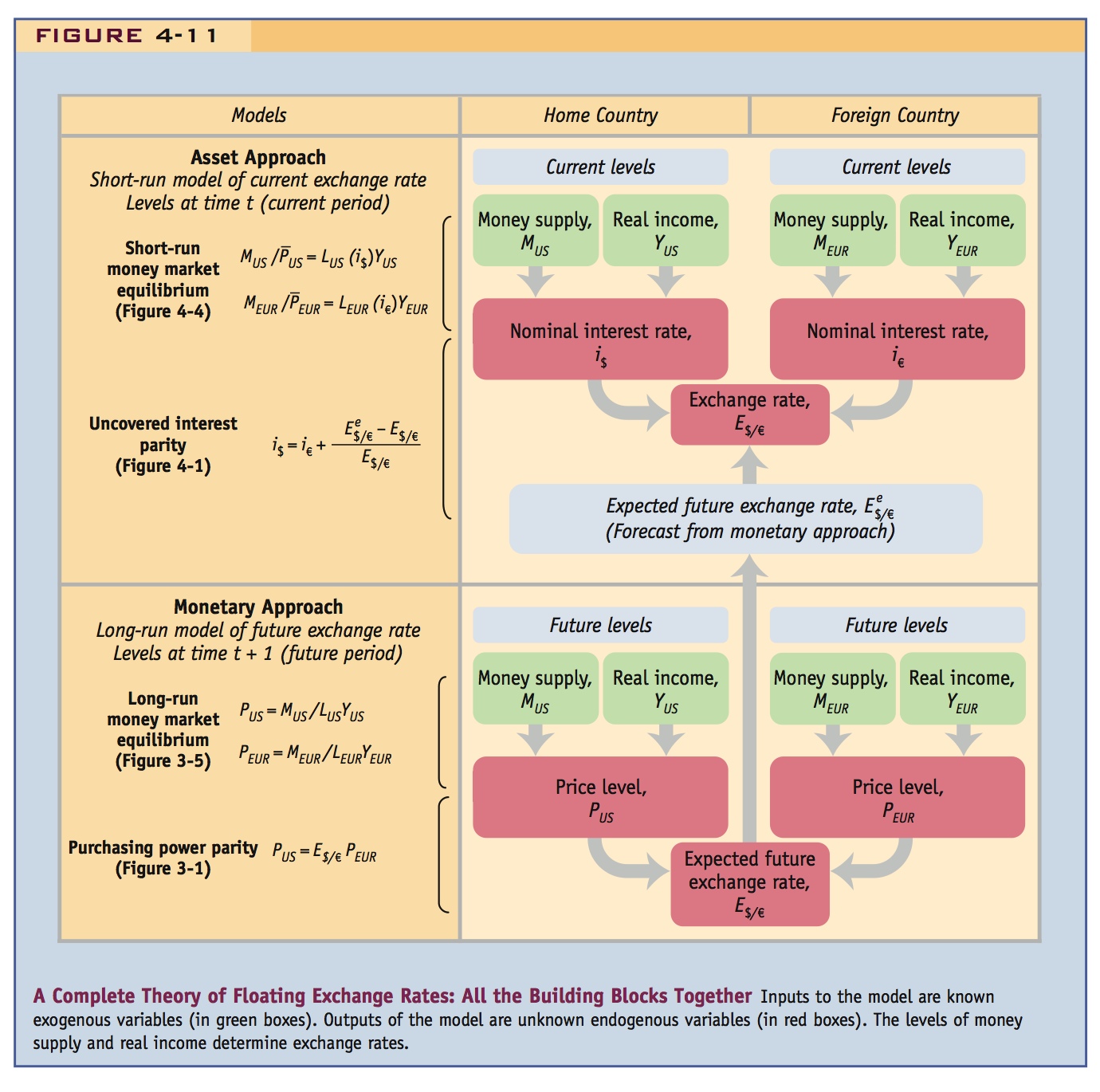
Our analysis is shown Figure 4-12. Panels (a) and (b) show the short-run impacts of a permanent increase in the money supply in the home (U.S.) money and FX markets; panels (c) and (d) show the long-run impacts and the adjustment from the short run to the long run.
As shown in panels (a), (b), (c), and (d), we suppose the home economy starts with initial equilibria in the home money and FX markets shown by points 1 and 1′, respectively. In the money market, in panels (a) and (c), at point 1, the home money market is initially in equilibrium: MS1 corresponds to an initial real money supply of  ; given real money demand MD, the nominal interest rate is
  . In the FX market, in panels (b) and (d), at point 1′, the domestic return DR1 is the nominal interest rate . Given the foreign return curve FR1, the equilibrium exchange rate is
  . If both economies are at a long-run equilibrium with zero depreciation, then this is also the expected future exchange rate
  .
.
Students will find this really exciting once they get it, but work through it slowly. Everything going on in Figure 4-12 can also be expressed using a more complicated version of the flow chart mentioned in a previous comment. This will help them parse out the causal links. Use different colors to distinguish between current and future changes, and show the latter feeds back to the former via Ee.
We now start to figure out what happens after the policy shock hits today, working backward from the future to the present.
The Long Run Refer to panels (c) and (d) of Figure 4-12. In the long run, we know from the monetary approach that an increase in the money supply will eventually lead to a proportionate increase in the price level and the exchange rate. If the money supply increases from  to
to  today, then the price level will eventually increase by the same proportion from
  to
to  , and, to maintain PPP, the exchange rate will eventually rise by the same proportion (and the dollar will depreciate) from to its long-run level
  , in panel (d), where
  . (We use “4” to denote long-run exchange rate values because there will be some short-run responses to consider in just a moment.)
Thus, in the long run, in panel (c), if money and prices both rise in the same proportion, then the real money supply will be unchanged at its original level 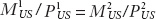 , the real money supply curve will still be in its original position MS1, and the nominal interest rate will again be . In the long run, the money market returns to where it started: long-run equilibrium is at point 4 (which is the same as point 1).
In the FX market, however, a permanent money supply shock causes some permanent changes in the long run. One thing that does not change is the domestic return DR1, since in the long run it returns to . But the exchange rate will rise from the initial long-run exchange rate , to a new long-run level . Because is a long-run stable level, it is also the new expected level of the exchange rate that will prevail in the future. That is, the future will look like the present, under our assumptions, except that the exchange rate will be sitting at instead of . What does this change do to the foreign return curve FR? As we know, when the expected exchange rate increases, foreign returns are higher, so the FR curve shifts up, from FR1 to FR2. Because in the long run is the new stable equilibrium exchange rate, and is the interest rate, the new FX market equilibrium is at point 4′ where FR2 intersects DR1.
136
137
The Short Run Only now that we have changes in expectations worked out can we work back through panels (a) and (b) of Figure 4-12 to see what will happen in the short run.
Look first at the FX market in panel (b). Because expectations about the future exchange rate have changed with today’s policy announcement, the FX market is affected immediately. Everyone knows that the exchange rate will be in the future. The foreign return curve shifts when the expected exchange rate changes; it rises from FR1 to FR2. This is the same shift we just saw in the long-run panel (d). The dollar is expected to depreciate to (relative to ) in the future, so euro deposits are more attractive today.
Now consider the impact of the change in monetary policy in the short run. Look at the money market in panel (a). In the short run, if the money supply increases from to but prices are sticky at , then real money balances rise from to  . The real money supply shifts from MS1 to MS2 and the home interest rate falls from to
  , leading to a new short-run money market equilibrium at point 2.
Now look back to the FX market in panel (b). If this were a temporary monetary policy shock, expectations would be unchanged, and the FR1 curve would still describe foreign returns, but domestic returns would fall from DR1 to DR2 as the interest rate fell and the home currency would depreciate to the level  . The FX market equilibrium, after a temporary money supply shock, would be at point 3′, as we have seen before.
But this is not the case now. This time we are looking at a permanent shock to money supply. It has two effects on today’s FX market. One impact of the money supply shock is to lower the home interest rate, decreasing domestic returns in today’s FX market from DR1 to DR2. The other impact of the money supply shock is to increase the future expected exchange rate, increasing foreign returns in today’s FX market from FR1 to FR2. Hence, the FX market equilibrium in the short run is where DR2 and FR2 intersect, now at point 2′, and the exchange rate depreciates all the way to  .
.
Note that the short-run equilibrium level of the exchange rate () is higher than the level that would be observed under a temporary shock () and also higher than the level that will be observed in the long run (). To sum up, in the short run, the permanent shock causes the exchange rate to depreciate more than it would under a temporary shock and more than it will end up depreciating in the long run.
Adjustment from Short Run to Long Run The arrows in panels (c) and (d) of Figure 4-12 trace what happens as we move from the short run to the long run. Prices that were initially sticky in the short run become unstuck. The price level rises from to , and this pushes the real money supply back to its initial level, from MS2 back to MS1. Money demand MD is unchanged. Hence, in the home money market of panel (c), the economy moves from the short-run equilibrium at point 2 to the long-run equilibrium, which is again at point 1, following the path shown by the arrows. Hence, the interest rate gradually rises from back to . This raises the domestic returns over in the FX market of panel (d) from DR2 back to DR1. So the FX market moves from the short-run equilibrium at point 2′ to the long-run equilibrium, which is again at point 4′.
An Example Let’s make this very tricky experiment a bit more concrete with a numerical example. Suppose you are told that, all else equal, (i) the home money supply permanently increases by 5% today; (ii) prices are sticky in the short run, so this also causes an increase in real money supply that lowers domestic interest rates by four percentage points from 6% to 2%; (iii) prices will fully adjust in one year’s time to today’s monetary expansion and PPP will hold again. Based on this information, can you predict what will happen to prices and the exchange rate today and in a year’s time?
138
Yes. Work backward from the long run to the short run, as before. In the long run, a 5% increase in M means a 5% increase in P that will be achieved in one year. By PPP, this 5% increase in P implies a 5% rise in E (a 5% depreciation in the dollar’s value) over the same period. In other words, over the next year E will rise at 5% per year, which will be the rate of depreciation. Finally, in the short run, UIP tells us what happens to the exchange rate today: to compensate investors for the four percentage point decrease in the domestic interest rate, arbitrage in the FX market requires that the value of the home currency be expected to appreciate at 4% per year; that is, E must fall 4% in the year ahead. However, if E has to fall 4% in the next year and still end up 5% above its level at the start of today, then it must jump up 9% today: it overshoots its long-run level.
Overshooting
Compared with the temporary expansion of money supply we studied before, the permanent shock has a much greater impact on the exchange rate in the short run.
Under the temporary shock, domestic returns go down; traders want to sell the dollar for one reason only—temporarily lower dollar interest rates make dollar deposits less attractive. Under the permanent shock, domestic returns go down and foreign returns go up; traders want to sell the dollar for two reasons—temporarily lower dollar interest rates and an expected dollar depreciation make dollar deposits much less attractive. In the short run, the interest rate and exchange rate effects combine to create an instantaneous “double whammy” for the dollar, which gives rise to a phenomenon that economists refer to as exchange rate overshooting.
Explain the double whammy to motivate overshooting. Increasing M has two effects: (1) Because prices are sticky it lowers interest rates, which depreciates the currency. (2) Because people expect depreciation in the future they sell the currency now, so there is an even larger depreciation.
Emphasize that overshooting requires two things, (1) sticky prices and (2) forward-looking behavior. Demonstrate that overshooting would not occur if either prices were flexible or if people did not anticipate the future.
To better visualize the overshooting phenomenon, we show in Figure 4-13 the time path over which the key economic variables change after the permanent shock we just studied using Figure 4-12. We see the following:
- The nominal money supply is subject to a one-time increase at time T.
- Real money balances rise instantaneously but revert to their initial level in the long run; the nominal interest rate falls instantaneously but reverts to its initial level in the long run.
- The price level is sticky in the short run but rises to a new higher level in the long run, increasing in the same proportion as the nominal money supply.
- The exchange rate rises (depreciates) to a new higher level in the long run, rising in the same proportion as the nominal money supply. In the short run, however, the exchange rate rises even more, overshooting its long-run level, then gradually decreasing to its long-run level (which is still higher than the initial level).
These graphs put it all together, and students like seeing how things unfold over time.
The overshooting result adds yet another argument for the importance of a sound long-run nominal anchor: without it, exchange rates are likely to be more volatile, creating instability in the forex market and possibly in the wider economy. The wild fluctuations of exchange rates in the 1970s, at a time when exchange rate anchors were ripped loose, exposed these linkages with great clarity (see Side Bar: Overshooting in Practice). And new research provides evidence that the shift to a new form of anchoring, inflation targeting, might be helping to bring down exchange rate volatility in recent years.3
139
140
We have discussed how volatile exchange rates are. Mention that Dornbusch provided a framework for explaining such large fluctuations in the context of a sticky-price Keynesian model with perfect foresight.
Describes the environment of highly volatile exchange rates after Bretton Woods that inspired Dornbusch to write his seminal paper.
Overshooting in Practice
Overshooting can happen in theory, but does it happen in the real world? The model tells us that if there is a tendency for monetary policy shocks to be more permanent than temporary, then there will be a tendency for the exchange rate to be more volatile. Thus, we might expect to see a serious increase in exchange rate volatility whenever a nominal anchoring system breaks down. Indeed, such conditions were seen in the 1970s, which is precisely when the overshooting phenomenon was discovered. How did this happen?
From the 1870s until the 1970s, except during major crises and wars, the world’s major currencies were fixed against one another. Floating rates were considered anathema by policy makers and economists. Later in this book, we study the gold standard regime that began circa 1870 and fizzled out in the 1930s and the subsequent “dollar standard” of the 1950s and 1960s that was devised at a conference at Bretton Woods, New Hampshire, in 1944. As we’ll see, the Bretton Woods system did not survive for various reasons.
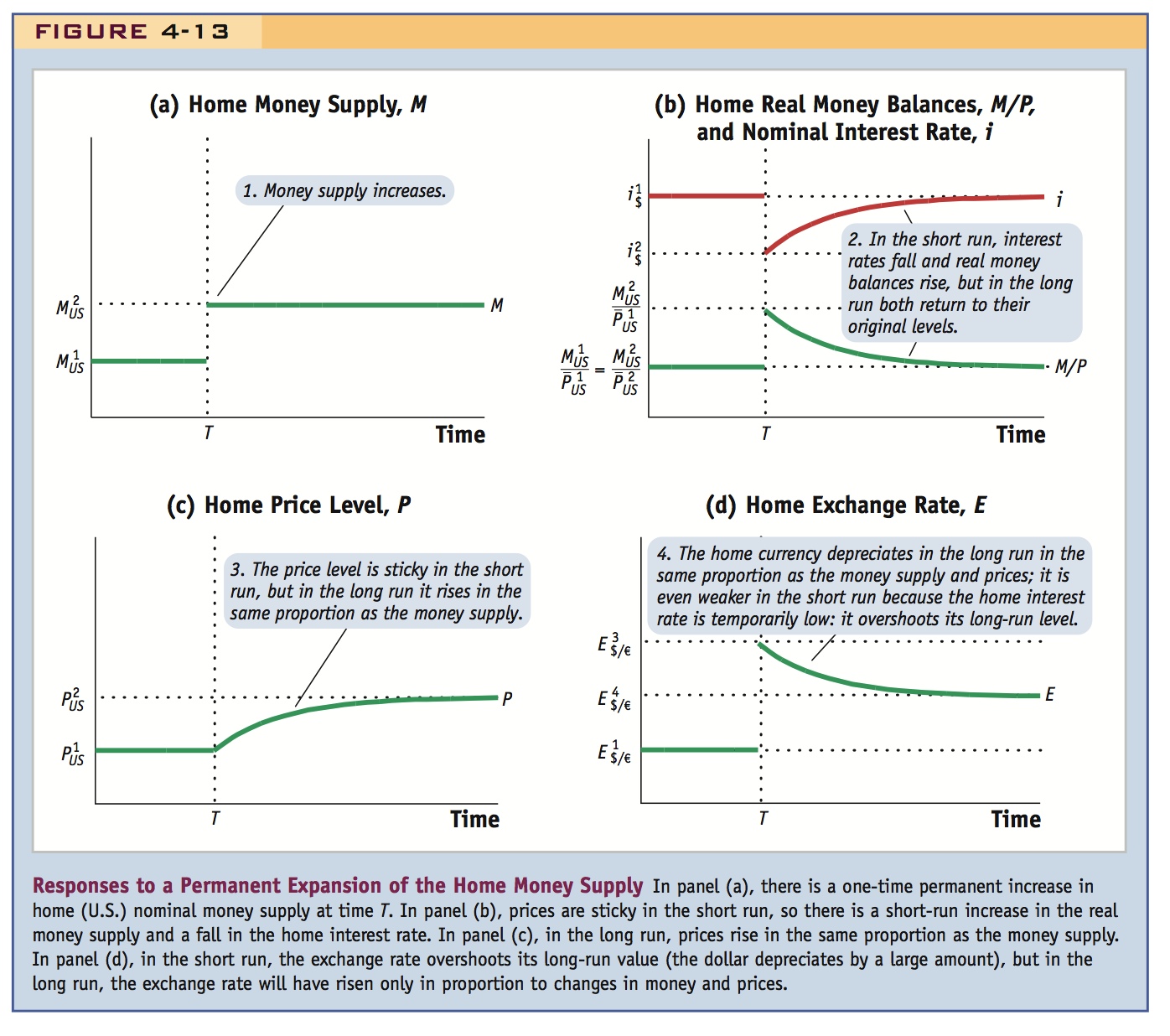
When floating rates reappeared in the 1970s, fears of instability returned. Concern mounted as floating exchange rates proved much more volatile than could be explained according to the prevailing flexible-price monetary approach: the models said that money supplies and real income were simply too stable to be able to generate such large fluctuations (as seen in Figure 4-14). Some feared that this was a case of animal spirits, John Maynard Keynes’s term for irrational forces, especially in asset markets like that for foreign exchange. The challenge to economists was to derive a new model that could account for the wild swings in exchange rates.
In 1976, economist Rudiger Dornbusch of the Massachusetts Institute of Technology developed such a model. Building on Keynesian foundations, Dornbusch showed that sticky prices and flexible exchange rates implied exchange rate overshooting.* Dornbusch’s seminal work was a rare case of a theory arriving at just the right time to help explain reality. In the 1970s, countries abandoned exchange rate anchors and groped for new ways to conduct monetary policy in a new economic environment. Policies varied and inflation rates grew, diverged, and persisted. Overshooting helps make sense of all this: if traders saw policies as having no well-defined anchor, monetary policy shocks might no longer be guaranteed to be temporary, so long-run expectations could swing wildly with every piece of news.
* Rudiger Dornbusch, December 1976, “Expectations and Exchange Rate Dynamics,” Journal of Political Economy, 84, 1161–1176.
141