3 Gains from Efficient Investment
Financial openness makes it easier for countries to invest and take advantage of new production opportunities.
1. The Basic Model
Introduce I, so that the LRBC is PV of Q = PV of C + PV of I. Again compare the closed economy with an open economy where the LRBC is satisfied.
2. Efficient Investment: A Numerical Example and Generalization
Suppose an investment opportunity occurs today. It requires a sacrifice of current Q and yields a permanent increase in Q thereafter. The closed economy would have to give up C today to undertake the investment. The open economy borrows today to finance the investment, running a trade deficit. It also enjoys a permanent increase in consumption, but to repay the debt it runs trade surpluses in perpetuity.
1. Generalizing
The model is similar to that in our discussion of consumption smoothing. The investment requires ΔK units of output today, and generates ΔQ units of output every period thereafter. Consumers want to maintain a constant consumption stream, constrained only by the LRBC. Given the PV of C, therefore, the economy wants to maximize PV of Q – PV of I. The investment costs ΔK today, and yields a perpetual increase in output with PV of ΔQ /r*. Therefore investment occurs up to the point where ΔQ = r* ΔK. Equivalently, optimal investment requires MPK = r* .
3.Summary: Make Hay While the Sun Shines
In a closed economy, investment requires the sacrifice of current consumption. In an open economy, however, the economy can borrow to finance investment, without sacrificing consumption. It will invest up to the point where the world interest rate equals the MPK.
Suppose an economy has opened up, and is taking full advantage of the gains from consumption smoothing. Has it completely exploited the benefits of financial globalization? The answer is no, because openness delivers gains not only on the consumption side but also on the investment side by improving a country’s ability to augment its capital stock and take advantage of new production opportunities.
The Basic Model
To illustrate these investment gains, we must refine the model we have been using by abandoning the assumption that output can be produced using only labor. We now assume that producing output requires labor and capital, which is created over time by investing output. When we make this change, the long-run budget constraint in Equation (6-4) must be modified to include investment I as a component of GNE. For simplicity, however, we still assume that government consumption G is zero. With this change, the LRBC becomes
221
You can probably just assert this, since it is such an obvious extension of the previous intertemporal budget constraint. Write the two period version.
Because the TB is output (Q) minus expenditure (C + I), we can rewrite this last equation in the following form:

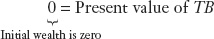
The LRBC will hold if and only if the present value of output Q equals the present value of expenditure (C + I).
Using this modified LRBC, we now study investment and consumption decisions in two cases:
- A closed economy, in which external borrowing and lending are not possible, the trade balance is zero in all periods, and the LRBC is automatically satisfied
- An open economy, in which borrowing and lending are possible, the trade balance can be more or less than zero, and we must verify that the LRBC is satisfied
The example of Chile’s sovereign wealth fund
Copper-Bottomed Insurance
Many developing countries experience output volatility. Sovereign wealth funds can buffer these shocks, as recent experience in Chile has shown.
Thousands of government workers marched on downtown Santiago [in November 2008], burning an effigy of Chilean Finance Minister Andres Velasco and calling him “disgusting” as a strike for higher wages paralyzed public services.
Five months later, polls show that Velasco is President Michelle Bachelet’s most popular minister. During a three-year copper boom he and central bank President Jose De Gregorio set aside $48.6 billion, more than 30 percent of the country’s gross domestic product, that he is now using for tax cuts, subsidies and cash handouts to poor families.
The Chilean peso has risen almost 10 percent against the dollar this year to become the best-performing currency among emerging markets. The country’s economy is expected to grow 0.1 percent in 2009, as the region contracts 1.5 percent, according to the International Monetary Fund….
Velasco, 48, applied the lessons learned from decades of economic failure in Latin America—ones he said could also help the U.S. The current crisis followed “a massive regulatory failure in many advanced financial markets over the last decade or so,” Velasco said in an interview April 21 [2009] in his office overlooking the presidential palace in downtown Santiago.
“This is a movie that may be novel to some Americans, but this is a movie that people in other places of the world, Chile included, know we have seen,” said Velasco, who is scheduled to meet April 25 with Federal Reserve Chairman Ben S. Bernanke in Washington. “We know how it begins, how it unfolds and how it ends.”…
Commodity-driven swings of boom and bust have defined Latin America’s economic history for the past 100 years.
“That is a cycle that needs to be ended,” Velasco said. “We have been out to show that a Latin American country can manage properly, and not mismanage, a commodity cycle. You save in times of abundance, and you invest in lean times.”
When Velasco joined Bachelet’s new cabinet in March 2006, the price of copper had risen by more than half in 12 months to $2.25 a pound. Taxes and profits from state-owned Codelco, the world’s largest copper producer, provide about 15 percent of government revenue. Bachelet, 57, Chile’s second consecutive socialist president, came under almost immediate pressure to start spending the revenue.
Students went on strike in May of that year, demanding more money for education. More than 800,000 people protested at high schools and universities, and police with water cannons and tear gas arrested more than 1,000. Velasco reiterated his commitment to “prudent fiscal policies” as politicians from the governing coalition demanded he resign….
In his first three years in office, Velasco posted the biggest budget surpluses since the country returned to democracy in 1990. In 2007, Chile became a net creditor for the first time since independence from Spain in 1810.
Last July [2008], copper reached a record of $4.08 a pound. By year-end, the central bank had built $23.2 billion of reserves. The government had $22.7 billion in offshore funds and about $2.8 billion in its own holdings.
After Lehman Brothers Holdings Inc.’s September 15 bankruptcy sparked a global credit freeze, Velasco and De Gregorio had the equivalent of more than 30 percent of GDP available if needed to shore up Chile’s banks and defend the peso.
The price of copper plummeted 52 percent from September 30 to year-end, and Velasco dusted off his checkbook. In the first week of January, he and Bachelet unveiled a $4 billion package of tax cuts and subsidies.
“He has been vindicated,” said Luis Oganes, head of Latin American research at JPMorgan Chase & Co. in New York, who studied under Velasco….
Velasco’s stimulus spending, including 40,000-peso ($68.41) handouts to 1.7 million poor families, has paid off politically. His approval rating almost doubled to 57 percent in March from a low of 31 percent in August…. He is now the most well-liked member of the government, second only to the president at 62 percent.
“People finally understood what was behind his ‘stinginess’ of early years,” said Sebastian Edwards, a Chilean economist at the University of California, Los Angeles. “That explains the rise in his popularity.”
Source: Excerpted from Sebastian Boyd, “Harvard Peso Doctor Vindicated as Chile Evades Slump,” bloomberg.com, April 23, 2009. Used with permission of Bloomberg L.P. © 2013. All rights reserved.
222
Efficient Investment: A Numerical Example and Generalization
Here too, it may be cleaner just to write down a two-period, neoclassical investment problem, where th firm wants to maximize the PV of production - Investment (the left-hand side of 17-5). Derive the result that you should invest as long as MPK > r* .
Let’s start with a country that has output of 100, consumption C of 100, no investment, a zero trade balance, and zero external wealth. If that state persisted, the LRBC would be satisfied, just as it was in the prior numerical example with consumption smoothing. This outcome describes the optimal path of consumption in both the closed and open economies when output is constant and there are no shocks, that is, nothing happens here that makes the country want to alter its output and consumption.
But now suppose there is a shock in year 0 that takes the form of a new investment opportunity. For example, it could be that in year 0 engineers discover that by building a new factory with a new machine, the country can produce a certain good much more cheaply than current technology allows. Or perhaps there is a resource discovery, but a mine must first be built to extract the minerals from the earth. What happens next? We turn first to a numerical example and then supply a more general answer.
We assume that the investment (in machines or factories or mines) would require an expenditure of 16 units, and that the investment will pay off in future years by increasing the country’s output by 5 units in year 1 and all subsequent years (but not in year 0).
The country now faces some choices. Should it make this investment? And if it does, will it make out better if it is open or closed? We find the answers to these questions by looking at how an open economy would deal with the opportunity to invest, and then showing why a country would make itself worse off by choosing to be closed, thereby relinquishing at least some of the gains the investment opportunity offers.
As in the previous example, the key to solving this problem is to work with the LRBC and see how the choices a country makes to satisfy it have to change as circumstances do. Before the investment opportunity shock, output and consumption were each 100 in all periods, and had a present value of 2,100. Investment was zero in every period, and the LRBC given by Equation (6-5) was clearly satisfied. If the country decides to not act on the investment opportunity, this situation continues unchanged whether the economy is closed or open.
223
Now suppose an open economy undertakes the investment. First, we must calculate the difference this would make to the country’s resources, as measured by the present value of output. Output would be 100 today and then 105 in every subsequent year. The present value of this stream of output is 100 plus 105/0.05 or 2,200. This is an increase of 100 over the old present value of output (2,100). The present value of the addition to output (of 5 units every subsequent period) is 100.
Can all of this additional output be devoted to consumption? No, because the country has had to invest 16 units in the current period to obtain this future stream of additional output. In this scenario, because all investment occurs in the current period, 16 is the present value of investment in the modified LRBC given by Equation (6-5).
Looking at that LRBC, we’ve calculated the present value of output (2,200), and now we have the present value of investment (16). We can see that the present value of consumption must equal 2,200 minus 16, or 2,184. This is 4% higher than it was without the investment. Even though some expenditure has to be devoted to investment, the resources available for consumption have risen by 4% in present value terms (from 2,100 without the investment, to 2,184 with it).
We can now find the new level of smooth consumption each period that satisfies the LRBC. Because the present value of C has risen by 4% from 2,100 to 2,184, the country can afford to raise consumption C in all periods by 4% from 100 to 104. (As a check, note that 104 + 104/0.05 = 2,184.) Is the country better off if it makes the investment? Yes—not only does its consumption remain smooth, but it is also 4% higher in all periods.
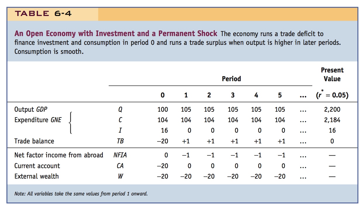
Table 6-4 lays out the details of this case. In year 0, consumption C is 104, investment I is 16, and GNE is 120. The trade balance is −20 because output Q is only 100. The country must borrow 20 units in year 0 to fund the investment of 16 and the 4 additional units of consumption the country can afford as a result of the investment. In all future years, consumption C is 104, and because there is no subsequent investment, GNE is also 104. Output Q is 105, and the trade balance is +1.
224
The initial trade deficit of 20 in year 0 results in an external debt of 20. As a perpetual loan, with an interest rate of 5%, this debt of 20 must be serviced by net interest payments of −1 in each subsequent year if the LRBC is to be satisfied. The interest payment of −1 offsets the trade surplus of +1 each period forever. Hence, the current account is zero in all future years, with no further borrowing, and the country’s external wealth is −20 in all periods. External wealth does not explode, and the LRBC is satisfied.
This outcome is preferable to any outcome a closed economy can achieve. To attain an output level of 105 from year 1 on, a closed economy would have to cut consumption to 84 in year 0 to free up 16 units for investment. Although the country would then enjoy consumption of 105 in all subsequent years, this is not a smooth consumption path! The open economy could choose this path (cutting consumption to 84 in year 0), because it satisfies the LRBC. It won’t choose this path, however, because by making the investment in this way, it cannot smooth its consumption and cannot smooth it at a higher level. The open economy is better off making the investment and smoothing consumption, two goals that the closed economy cannot simultaneously achieve.
Generalizing The lesson of our numerical example applies to any situation in which a country confronts new investment opportunities. Suppose that a country starts with zero external wealth, constant output Q, consumption C equal to output, and investment I equal to zero. A new investment opportunity appears requiring ΔK units of output in year 0. This investment will generate an additional ΔQ units of output in year 1 and all later years (but not in year 0).
Ultimately, consumers care about consumption. In an open economy, they can smooth their consumption, given future output. The constant level of consumption is limited only by the present value of available resources, as expressed by the LRBC. Maximizing the level of consumption is the same as maximizing the present value of consumption. Rearranging Equation (6-5), the LRBC requires that the present value of consumption must equal the present value of output minus the present value of investment. How is this present value maximized?
The increase in the present value of output PV(Q) comes from extra output in every year but year 0, and the present value of these additions to output is, using Equation (6-2),

The change in the present value of investment PV(I) is simply ΔK.
This means the investment will increase the present value of consumption—and hence will be undertaken—if and only if ΔQ/r* ΔK. There are two ways to look at this conclusion. Rearranging, investment is undertaken when
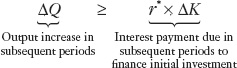
The intuition here is that investment occurs up to the point at which the annual benefit from the marginal unit of capital (ΔQ) equals or exceeds the annual cost of borrowing the funds to pay for that capital (r*ΔK).
225
Putting it another way, dividing by ΔK, investment is undertaken when
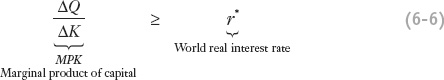
This is a standard formula for the optimal or efficient level of investment and may look familiar from other courses in economics. Firms will take on investment projects as long as the marginal product of capital (MPK) is at least as great as the real interest rate.
Summary: Make Hay While the Sun Shines
In an open economy, firms borrow and repay to undertake investment that maximizes the present value of output. Households also borrow and lend to smooth consumption, but these borrowing and lending decisions are separate from those of firms.
This is the Fisher separation theorem, separating the investment and saving decisions. It may be hard for students to see what this is actually saying without the benefit of the two-period model--but developing the full two-period model with a concave intertemporal PPF may be asking too much.
On the other hand, developing such a model would have the merit of showing that the gains from international intertemporal trade are isomorphic to the gains from trade in goods and services in a single time period.
Again, a simple phrase to use that captures the gist of the argument.
When investing, an open economy sets its MPK equal to the world real rate of interest. If conditions are unusually good (high productivity), it makes sense to invest more capital and produce more output. Conversely, when conditions turn bad (low productivity), it makes sense to lower capital inputs and produce less output. This strategy maximizes the present value of output minus investment. Households then address the separate problem of how to smooth the path of consumption when output changes. A closed economy must be self-sufficient. Any resources invested are resources not consumed. More investment implies less consumption. This creates a trade-off. When investment opportunities are good, the country wants to invest to generate higher output in the future. Anticipating that higher output, the country wants to consume more today, but it cannot—it must consume less to invest more.
Proverbially, financial openness helps countries to “make hay while the sun shines”—and, in particular, to do so without having to engage in a trade-off against the important objective of consumption smoothing. The lesson here has a simple household analogy. Suppose you find a great investment opportunity. If you have no financial dealings with the outside world, you would have to sacrifice consumption and save to finance the investment.
Consider the example of the Norwegian oil boom, where I was financed entirely by borrowing from abroad, rather than by domestic savings. Does access to international capital decouple S and I in general? The evidence here suggests that the decoupling is greatest in economies where international financial integration has advanced the most.
1. Can Poor Countries Gain from Financial Globalization?
If a country’s MPK exceeds it should run TB deficits to finance I. Why then doesn’t more capital flow to poor countries?
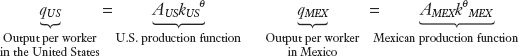
a. Production Function Approach
Use a Cobb-Douglas production function with capital share of 1/3.
b. A Benchmark Model: Countries Have Identical Productivity Levels
Set total factor productivity A = 1. Poorer countries must have higher MPKs than rich countries. Example: Mexican MPK in the 1980s was 5.4 times larger than the U.S. MPK. Then capital should flow from rich to poor countries until MPKs equalize. Output per worker should converge.
c. The Lucas Paradox: Why Doesn’t Capital Flow from Rich to Poor Countries?
Lucas’s question: Capital is not flowing from rich to poor countries?
d. An Augmented Model: Countries Have Different Productivity Levels
Answer: As are lower in poorer countries than in rich. Example: Mexican TFP must be 63 percent of the U.S.’s. This also implies that output per worker need not converge.
Delinking Saving from Investment
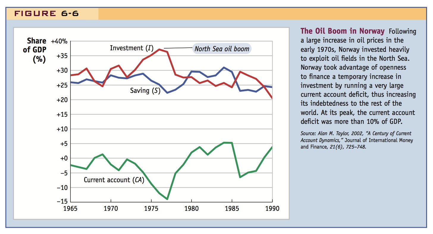
The story of the Norwegian oil boom provides a good illustration of our theory about investment and financial openness. North Sea oil was discovered in the 1960s, but the mass exploitation of this resource was unprofitable because cheap and plentiful supplies of oil were being produced elsewhere, primarily in the Persian Gulf. Then came the first “oil shock” in the early 1970s, when the cartel of Oil Producing and Exporting Countries (OPEC) colluded to raise world oil prices dramatically, a shock that was (correctly) viewed as permanent. At these higher oil prices, it suddenly made sense to exploit North Sea oil. Starting in the early 1970s, oil platforms, pipelines, refineries, and terminals were sprouting offshore and along the coast of Norway, causing its capital stock to permanently increase in response to a new productive investment opportunity.
226
Figure 6-6 shows the path of saving (S) and investment (I) measured as ratios of GDP in Norway from 1965 to 1990. The oil boom is clearly visible in the investment share of GDP, which in the 1970s rose about 10 percentage points above its typical level. Had Norway been a closed economy, this additional investment would have been financed by a decrease in the share of output devoted to public and private consumption. As you can see, no such sacrifice was necessary. Norway’s saving rate was flat in this period or even fell slightly. In Norway’s open economy, saving and investment were delinked and the difference was made up by the current account, CA = S − I, which moved sharply into deficit, approaching minus 15% of GDP at one point. Thus, all of the short-run increase in investment was financed by foreign investment in Norway, much of it by multinational oil companies.
Is Norway a special case? Economists have examined large international datasets to see whether there is general evidence that countries can delink investment decisions from saving decisions as the Norwegians did. One approach follows the pioneering work of Martin Feldstein and Charles Horioka.12 They estimated what fraction β of each additional dollar saved tended to be invested in the same country. In other words, in their model, if saving rose by an amount ΔS, they estimated that investment would rise by an amount ΔI = βΔS. In a closed economy, the “savings retention” measure β would equal 1, but they argued that increasing financial openness would tend to push β below 1.
For example, suppose one were to estimate β for the period 1980 to 2000 for three groups of countries with differing degrees of financial integration within the group: in a sample of countries in the European Union, where international financial integration had advanced furthest, the estimated value of β is 0.26, meaning that 26% of each additional dollar saved tended to be invested in the same country; in a sample of all developed countries with a somewhat lower level of financial integration, the estimate of β is 0.39; and in a sample of emerging markets, where financial integration was lower still, the estimate of β is 0.67.13 These data thus indicate that financially open countries seem to have a greater ability to delink saving and investment, in that they have a much lower “savings retention” measure β.
Discuss this: The original F-H paradox-- that beta was large--was interpreted as evidence against integration. But breaking it down by country types in this way suggests that in fact delinking of S and I is greater for financially open economies.
227
Can Poor Countries Gain from Financial Globalization?
Our analysis shows that if the world real interest rate is r* and a country has investment projects for which the marginal product of capital MPK exceeds r*, then the country should borrow from the rest of the world to finance investment in these projects. Keep this conclusion in mind as we now examine an enduring question in international macroeconomics: Why doesn’t more capital flow to poor countries?
They will be familiar with production function and diminishing marginal productivity, but may need to walk through the Cobb-Douglas example.
Production Function Approach To look at this question carefully, economists must take a stand on what determines a country’s marginal product of capital. For this purpose, economists usually employ a version of a production function that maps available capital per worker, k = K/L, and the prevailing level of productivity A to the level of output per worker, q = Q/L, where Q is GDP.
A simple and widely used production function takes the form
In fact, you may not need to get involved in the details of Cobb-Douglas at all. Just write q = Af(k) and draw Figure 6-7 (a). Depict the interest rates in the two countries as the slopes of the production at those two points and argue the profitability of capital flow to the poor country.
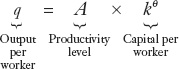
where θ is a number between 0 and 1 that measures the contribution of capital to production.14 Specifically, θ is the elasticity of output with respect to capital (i.e., a 1% increase in capital per worker generates a θ% increase in output per worker). In the real world, θ has been estimated to be approximately one-third, and this is the value we employ here.15 An illustration is given in the top part of Figure 6-7, panel (a), which graphs the production function for the case in which θ = 1/3 and the productivity level is set at a reference level of 1, so A = 1. Thus, for this case q = k1/3.
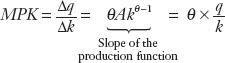
With this production function, what is the marginal product of capital, MPK? It is the slope of the production function, the incremental change in output per worker Δq divided by the incremental change in capital per worker Δk. As we can see from the figure, capital’s marginal product MPK (the extra output we get by increasing capital per worker) decreases as k increases. Indeed, from the preceding formula, we can find that MPK, or the slope of the production function, is given by
228
Thus, in this special case, the marginal product of capital is proportional to output per worker divided by capital per worker (the output–capital ratio) or the average product of capital. The MPK for the case we are studying, in which θ = 1/3 and A = 1, is shown in the bottom part of Figure 6-7, panel (a).
229
A Benchmark Model: Countries Have Identical Productivity Levels To see how a country responds to the possibilities opened up by financial globalization, let’s look at what determines the incentive to invest in small open economies of the type we are studying, assuming they all have access to the same level of productivity, A = 1.
To understand when such a country will invest, we need to understand how its MPK changes as k changes. For example, suppose the country increases k by a factor of 8. Because q = k1/3, q increases by a factor of 2 (the cube root of 8). Let’s suppose this brings the country up to the U.S. level of output per worker. Because MPK = θ × q/k and because q has risen by a factor of 2, while k has risen by a factor of 8, MPK changes by a factor of 1/4; that is, it falls to one-fourth its previous level.
This simple model says that poor countries with output per worker of one-half the U.S. level have an MPK of four times the U.S level. Countries with one-quarter the U.S. per worker output level have an MPK of 16 times the U.S level, and so on.
To make the model concrete, let’s see how well it applies to a comparison of the United States and Mexico in the late 1980s.16 During this time, the United States produced approximately twice as much GDP per worker as Mexico. Now let’s choose units such that all U.S. variables take the value 1, and Mexican variables are proportions of the corresponding U.S. variables. For example, with these units, q was 0.43 in Mexico in the late 1980s (i.e., output per worker in Mexico was 43% of output per worker in the United States).
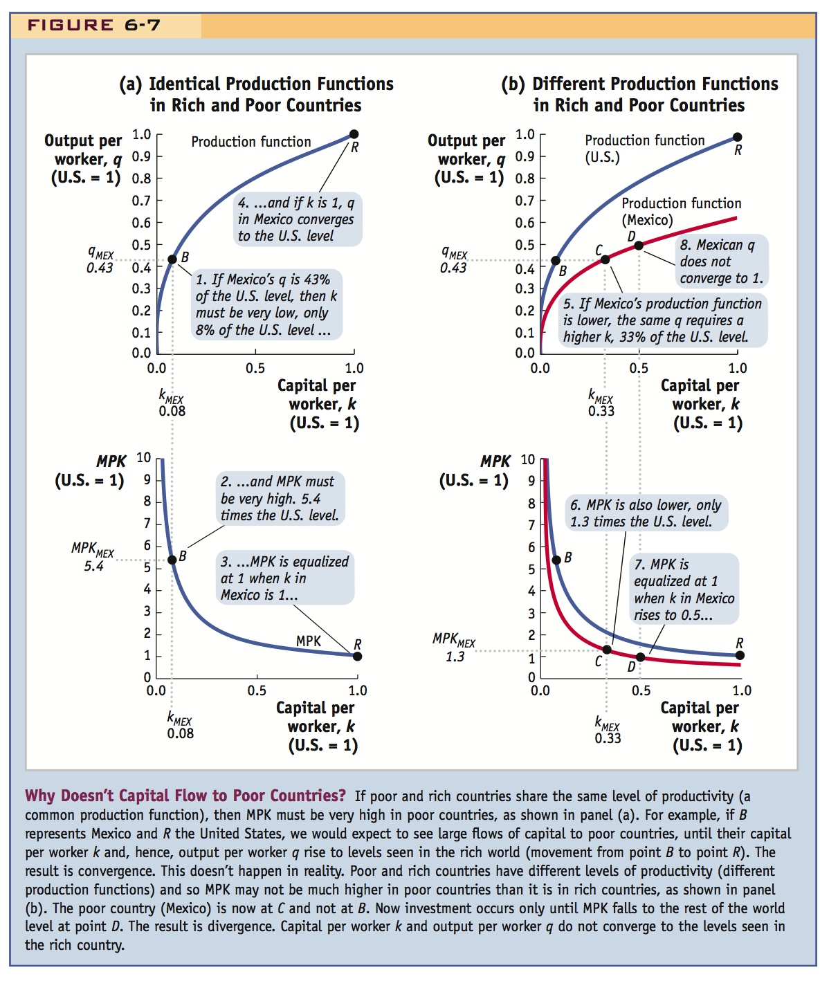
Now consider the implications of assuming that the economies of Mexico and the United States were described by the same production function with a common productivity level, A = 1. In Figure 6-7, panel (a), the United States is at point R (for rich) and Mexico is at point B, and its low output implies a capital per worker k that is only 8% of the U.S. level. What is Mexico’s marginal product of capital? It is 5.4 times the U.S. marginal product of capital. Why? As above, MPK is θ (a constant for both countries equal to 1/3) times q/k. In the United States, q/k = 1; in Mexico, q/k = 0.43/0.08 = 5.4.
Compare this to the argument in Chapter 3 that in the long run real interest rates should equalize.
We can think of the United States and other rich countries as representing the rest of the world—a large financially integrated region, from Mexico’s point of view. The world real interest rate r* is the opportunity cost of capital for the rest of the world, that is, the rich world’s MPK. If the real interest rate r* is, say, 10% in rich countries like the United States, then their MPK is 10%, and Mexico has an MPK of 54%!
To take an even more dramatic example, we could look at India, a much poorer country than Mexico. India’s output per worker was just 8.6% of the U.S. level in 1988. Using our simple benchmark model, we would infer that the MPK in India was 135 times the U.S. level!17
To sum up, the simple model says that the poorer the country, the higher its MPK, because of the twin assumptions of diminishing marginal product and a common productivity level. Investment ought to be very profitable in Mexico (and India, and all poor countries). Investment in Mexico should continue until Mexico is at point R. Economists would describe such a trajectory for Mexico as convergence. If the world is characterized by convergence, countries can reach the level of capital per worker and output per worker of the rich country through investment and capital accumulation alone.
230
The Lucas Paradox: Why Doesn’t Capital Flow from Rich to Poor Countries? Twenty or thirty years ago, a widespread view among economists was that poor countries had access to exactly the same technologies as rich countries, given the flow of ideas and knowledge around a globalizing world. This led economists to assume that if policies shifted to allow greater international movement of capital, foreign investment would flood into poor countries because their very poverty implied that capital was scarce in these countries, and therefore its marginal product was high.
But as Nobel laureate Robert Lucas wrote in his widely cited article “Why Doesn’t Capital Flow from Rich to Poor Countries?”:
Say that is one of the great issues in growth economics.
If this model were anywhere close to being accurate, and if world capital markets were anywhere close to being free and complete, it is clear that, in the face of return differentials of this magnitude, investment goods would flow rapidly from the United States and other wealthy countries to India and other poor countries. Indeed, one would expect no investment to occur in the wealthy countries…. The assumptions on technology and trade conditions that give rise to this example must be drastically wrong, but exactly what is wrong with them, and what assumptions should replace them?18
What was drastically wrong was the assumption of identical productivity levels A across countries, as represented by the single production function in Figure 6-7, panel (a)? Although this model is often invoked, it is generally invalid. Can we do better?
An Augmented Model: Countries Have Different Productivity Levels To see why capital does not flow to poor countries, we now suppose that A, the productivity level, is different in the United States and Mexico, as denoted by country subscripts:
Here too you may not need Cobb-Douglas; just let there be different A's.
Countries have potentially different production functions and different MPK curves, depending on their relative levels of productivity, as shown in Figure 6-7, panel (b). The Mexican curves are shown here as lower than the U.S. curves. We now show that this augmented model is a much better match with reality.
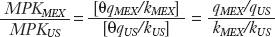
The earlier MPK equation holds for each country, so we can compute the ratios of country MPKs as
231
Using this equation, we can see the importance of allowing productivity levels to differ across countries. We know that qMEX/qUS = 0.43, but we can also obtain data on capital per worker that show kMEX/kUS = 0.33. If we plug these numbers into the last expression, we find that MPK in Mexico is not 5.4 times the U.S. level, as we had earlier determined, but only about 1.3 times (0.43/0.33) the U.S. level. The smaller multiple is due to the lower productivity level that our revised model reveals in Mexico.
A striking result.
Put another way, the data show that Mexico’s capital per worker is about one-third that of the United States. If the simple model were true, Mexico would have a level of output level per worker of (1/3)1/3 = 0.69 or 69% of the U.S. level. However, Mexico’s output per worker was much less, only 0.43 or 43% of the U.S. level. This gap can only be explained by a lower productivity level in Mexico. We infer that A in Mexico equals 0.43/0.69 = 0.63, or 63% of that in the United States.
This means that Mexico’s production function and MPK curves are lower than those for the United States. This more accurate representation of reality is shown in Figure 6-7, panel (b). Mexico is not at point B, as we assumed in panel (a); it is at point C, on a different (lower) production function and a different (lower) MPK curve. The MPK gap between Mexico and the United States is much smaller, which greatly reduces the incentive for capital to migrate to Mexico from the United States.
The measured MPK differentials in the augmented model do not seem to indicate a major failure of global capital markets to allocate capital efficiently. But the augmented model has very different implications for convergence. Mexico would borrow only enough to move from point C to point D, where its MPK equals r*. This investment would raise its output per worker a little, but it would still be far below that of the United States.
Profound conclusion: Productivity differences should cause divergence. Access to capital markets will not be sufficient for poor countries to catch up. But what is A, exactly? Not just technical efficiency. It may also reflect institutions, public policies, cultural conditions, and human capital.
e. More Bad News?
Other reasons to think convergence may not occur: (1) Poor countries face risk premia that (2) may be large enough to make capital flow to rich countries; (3) the cost of capital may be higher in poor countries; (4) capital’s share may be smaller in poor countries; (5) foreign aid shouldn’t be any more effective than private capital flows in promoting growth (unless they finance public goods that confer externalities sufficiently large to allow the economy to escape a “poverty trap”).
But there still might be conditional convergence.
Elicit discussion about the implications of rich countries converging to a nice steady state, and poor countries converging to another.
Students will have been posing that question before this point.
Discuss these two interpretations of A.
Also discuss these confounding factors. What if capital is flowing uphill?
A Versus k
In our previous calculations, we found that Mexico did not have a high level of MPK relative to the United States. Hence, we would not expect large flows of capital into Mexico but would expect Mexico to remain relatively poor even with access to global financial markets.
Is this conclusion true in general? What about other developing countries? Table 6-5 repeats the same exercise we just did for many developing countries, including Mexico. In all cases, predicted GDP gains due to financial globalization are large with the benchmark model, but disappointingly small once we augment the model to correct for productivity differences. Moreover, if we were to allow for the fact that gross national income (GNI) gains are less than GDP gains as a result of factor payments to foreign capital that would be due on foreign investment, then the net GNI gains would be smaller still.
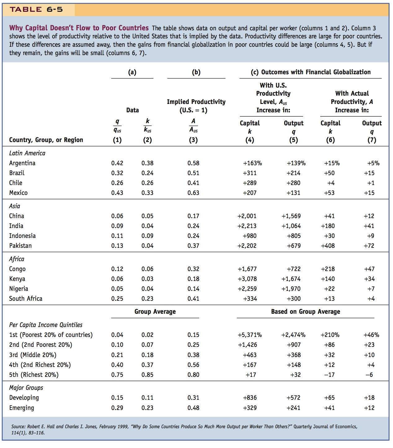
This is a profound result. Once we allow for productivity differences, investment will not cause poor countries to reach the same level of capital per worker or output per worker as rich countries. Economists describe this outcome as one of long-run divergence between rich and poor countries. Unless poor countries can lift their levels of productivity (raise A), access to international financial markets is of limited use. They may be able to usefully borrow capital, thereby increasing output per worker by some amount, but there are not enough opportunities for productive investment for complete convergence to occur.
232
In the developing world, global capital markets typically are not failing. Rather, low levels of productivity A make investment unprofitable, leading to low output levels that do not produce convergence. But what exactly does A represent?
233
An older school of thought focused on A as reflecting a country’s technical efficiency, construed narrowly as a function of its technology and management capabilities. Today, many economists believe there is very little blocking the flow of such knowledge between countries, and that the problem must instead be one of implementation. These economists believe that the level of A may primarily reflect a country’s social efficiency, construed broadly to include institutions, public policies, and even cultural conditions such as the level of trust. Low productivity might then follow from low levels of human capital (poor education policies) or poor-quality institutions (bad governance, corruption, red tape, and poor provision of public goods including infrastructure). And indeed there is some evidence that, among poorer countries, more capital does tend to flow to the countries with better institutions.19
More Bad News? The augmented model shows that as long as productivity gaps remain, investment will be discouraged, and, regrettably, poor countries will not see their incomes converge to rich levels. If we now take some other factors into account, the predictions of the model about convergence are even less optimistic.
- The model makes no allowance for risk premiums. Suppose the MPK is 10% in the United States and 13% in Mexico. The differential may be a risk premium Mexico must pay to foreign lenders that compensates them for the risk of investing in an emerging market (e.g., risks of regulatory changes, tax changes, expropriation, and other political risks). In this case, no additional capital flows into Mexico. In Figure 6-7, panel (b), Mexico stays at point C and its income does not increase at all.
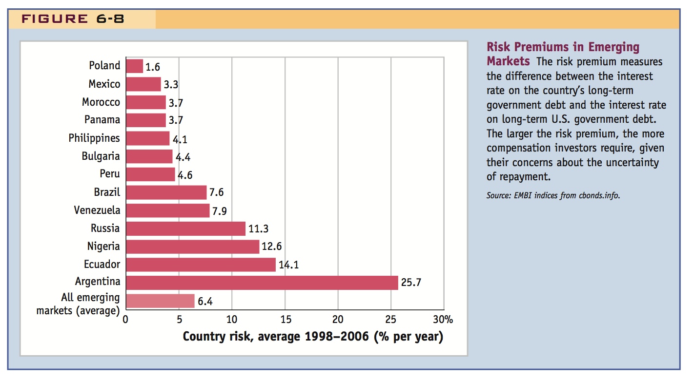
- Risk premiums may be large enough to cause capital to flow “uphill” from poor to rich. If world capital markets impose a risk premium higher than 3%, say, 7%, then capital would actually leave Mexico for the United States, moving from the higher to the lower MPK region, in search of a “safe haven” that provides higher risk-adjusted returns. In Figure 6-7, panel (b), Mexico would move left of point C as capital flowed out, and per capita output would fall. Is this a relevant case? Yes. Figure 6-8 shows that risk premiums can be substantial in emerging markets, including Mexico. And U.S. Treasury securities data indicate that from 1994 to 2006, U.S. holdings of Mexican assets rose from $50 billion to $65 billion, but Mexican holdings of U.S. assets rose from $5 billion to $95 billion; on net, capital moved north.
- The model assumes that investment goods can be acquired at the same relative price in output terms everywhere. In fact, the model treats one unit of investment as the same as one unit of output. But in developing countries, it often costs much more than one unit of output to purchase one unit of capital goods. Poor countries often are ill-equipped to efficiently supply nontraded capital goods (such as buildings or bridges), and their imported capital goods (such as machinery and equipment) are often quite expensive because of trade costs (such as tariffs and transport costs).20
- The model assumes that the contribution of capital to production is equal across countries. In our estimates, we used 1/3 as the elasticity of output with respect to capital. But recent research suggests that capital’s share may be much lower in many developing countries, where a large part of GDP is derived from natural resources with little use of physical capital. This lowers the MPK even more.21
- The model suggests that foreign aid may do no better than foreign investors in promoting growth. The model doesn’t care where additional capital comes from. Investments paid for by transfers (aid or debt relief) rather than private investments face the same low MPK and the same divergence result holds. Economists dispute whether foreign aid can make a difference to long-term development and growth, or if it is only an act of charity to prop up the poor (or even a total waste of money). The argument also extends to nonmarket and preferential lending offered to poor countries by international financial institutions such as the World Bank (see Side Bar: What Does the World Bank Do?). In support of the case that aid can make a difference, aid proponents argue that aid can finance public goods that can provide externalities sufficient to jolt a poor country out of a bad equilibrium or “poverty trap”—goods that private markets cannot provide (such as infrastructure, public health, and education). Aid skeptics reply that the evidence for such effects is weak, either because the links are not there or because in practice aid is so bureaucratized and subject to so many diversions and misappropriations that very little of it actually gets spent wisely (see Headlines: A Brief History of Foreign Aid).
235
Also entertain the possibility that human capital may be much greater in developed economies (up to 60 percent of the total capital stock in the U.S., by some estimates).
A primer on the World Bank
What Does the World Bank Do?
The World Bank (worldbank.org), based in Washington, D.C., is one of the Bretton Woods “twins” established in 1944 (the other is the International Monetary Fund). Its main arm, the International Bank for Reconstruction and Development, has 188 member countries. Its principal purpose is to provide financing and technical assistance to reduce poverty and promote sustained economic development in poor countries. A country’s voting weight in the governance of the World Bank is based on the size of its capital contributions. The World Bank can raise funds at low interest rates and issue AAA-rated debt as good as that of any sovereign nation. It then lends to poor borrowers at low rates. Because the borrower nations could not obtain loans on these terms (or even any terms) elsewhere, the loans are a form of aid or transfer. In return for the preferential rate, the bank may approve a loan for a particular development purpose (building infrastructure, for example) or to support a policy reform package. Controversially, conditions may also be imposed on the borrowing nation, such as changes in trade or fiscal policy. As a result of sovereignty, the implementation of the conditions and the use of the loans have in some cases not turned out as intended, although outright default on these preferential loans is almost unheard of.
The debate about the effectiveness of foreign aid and how it should be implemented
A Brief History of Foreign Aid
Foreign aid is frequently on the political agenda. But can it make any difference?
In 1985, when Bob Geldof organized the rock spectacular Live Aid to fight poverty in Africa, he kept things simple. “Give us your fucking money” was his famous (if apocryphal) command to an affluent Western audience—words that embodied Geldof’s conviction that charity alone could save Africa. He had no patience for complexity: we were rich, they were poor, let’s fix it. As he once said to a luckless official in the Sudan, after seeing a starving person, “I’m not interested in the bloody system! Why has he no food?”
Whatever Live Aid accomplished, it did not save Africa. Twenty years later, most of the continent is still mired in poverty. So when, earlier this month, Geldof put together Live 8, another rock spectacular, the utopian rhetoric was ditched. In its place was talk about the sort of stuff that Geldof once despised—debt-cancellation schemes and the need for “accountability and transparency” on the part of African governments—and, instead of fund-raising, a call for the leaders of the G-8 economies to step up their commitment to Africa. (In other words, don’t give us your fucking money; get interested in the bloody system.) Even after the G-8 leaders agreed to double aid to Africa, the prevailing mood was one of cautious optimism rather than euphoria.
That did not matter to the many critics of foreign aid, who mounted a lively backlash against both Live 8 and the G-8 summit. For them, continuing to give money to Africa is simply “pouring billions more down the same old rat-holes,” as the columnist Max Boot put it. At best, these critics say, it’s money wasted; at worst, it turns countries into aid junkies, clinging to the World Bank for their next fix. Instead of looking for help, African countries need to follow the so-called Asian Tigers (countries like South Korea and Taiwan), which overcame poverty by pursuing what Boot called “superior economic policies.”
Skepticism about the usefulness of alms to the Third World is certainly in order. Billions of dollars have ended up in the pockets of kleptocratic rulers—in Zaire alone, Mobutu Sese Soko stole at least four billion—and still more has been misspent on massive infrastructure boondoggles, like the twelve-billion-dollar Yacyreta Dam, between Argentina and Paraguay, which Argentina’s former President called “a monument to corruption.” And historically there has been little correlation between aid and economic growth.
This checkered record notwithstanding, it’s a myth that aid is doomed to failure. Foreign aid funded the campaign to eradicate smallpox, and in the sixties it brought the Green Revolution in agriculture to countries like India and Pakistan, lifting living standards and life expectancies for hundreds of millions of people. As for the Asian nations that Africa is being told to emulate, they may have pulled themselves up by their bootstraps, but at least they were provided with boots. In the postwar years, South Korea and Taiwan had the good fortune to become, effectively, client states of the U.S. Between 1946 and 1978, in fact, South Korea received nearly as much U.S. aid as the whole of Africa. Meanwhile, the billions that Taiwan got allowed it to fund a vast land-reform program and to eradicate malaria. And the U.S. gave the Asian Tigers more than money; it provided technical assistance and some military defense, and it offered preferential access to American markets.
236
Coincidence? Perhaps. But the two Middle Eastern countries that have shown relatively steady and substantial economic growth—Israel and Turkey—have also received tens of billions of dollars in U.S. aid. The few sub-Saharan African countries that have enjoyed any economic success at all of late—including Botswana, Mozambique, and Uganda—have been major aid recipients, as has Costa Rica, which has the best economy in Central America. Ireland (which is often called the Celtic Tiger) has enjoyed sizable subsidies from the European Union. China was the World Bank’s largest borrower for much of the past decade.
Nobody doubts that vast amounts of aid have been squandered, but there are reasons to think that we can improve on that record. In the first place, during the Cold War aid was more often a geopolitical tool than a well-considered economic strategy, so it’s not surprising that much of the money was wasted. And we now understand that the kind of aid you give, and the policies of the countries you give it to, makes a real difference. A recent study by three scholars at the Center for Global Development found that, on average, foreign aid that was targeted at stimulating immediate economic growth (as opposed to, say, dealing with imminent crises) has had a significantly beneficial effect, even in Africa.
There’s still a lot wrong with the way that foreign aid is administered. Too little attention is paid to figuring out which programs work and which don’t, and aid still takes too little advantage of market mechanisms, which are essential to making improvements last. There’s plenty we don’t know about what makes one country succeed and another fail, and, as the former World Bank economist William Easterly points out, the foreign-aid establishment has often promised in the past that things would be different. So we should approach the problem of aid with humility. Yet humility is no excuse for paralysis. In 2002, President Bush created the Millennium Challenge Account, which is designed to target assistance to countries that adopt smart policies, and said that the U.S. would give five billion dollars in aid by 2006. Three years later, a grand total of $117,500 has been handed out. By all means, let’s be tough-minded about aid. But let’s not be hardheaded about it.
Source: James Surowiecki, “A Farewell to Alms?” New Yorker, July 25, 2005.
This is a devastating and discouraging indictment.
Some efforts are now being made to ensure more aid is directed toward countries with better institutional environments: the U.S. Millennium Challenge Corporation has pursued this goal, as has the World Bank. But past evidence is not encouraging: an exhaustive study of aid and growth by economists Raghuram Rajan and Arvind Subramanian concluded: “We find little robust evidence of a positive (or negative) relationship between aid inflows into a country and its economic growth. We also find no evidence that aid works better in better policy or geographical environments, or that certain forms of aid work better than others. Our findings suggest that for aid to be effective in the future, the aid apparatus will have to be rethought.”22