4 Money Market Equilibrium: Deriving the LM Curve
LM depicts equilibrium in the money market.
1. Money Market Recap
Review of the money market to get to the equilibrium condition M⁄P = L(i)Y. If Y increases money demand increases, raising the interest rate.
2. Deriving the LM Curve
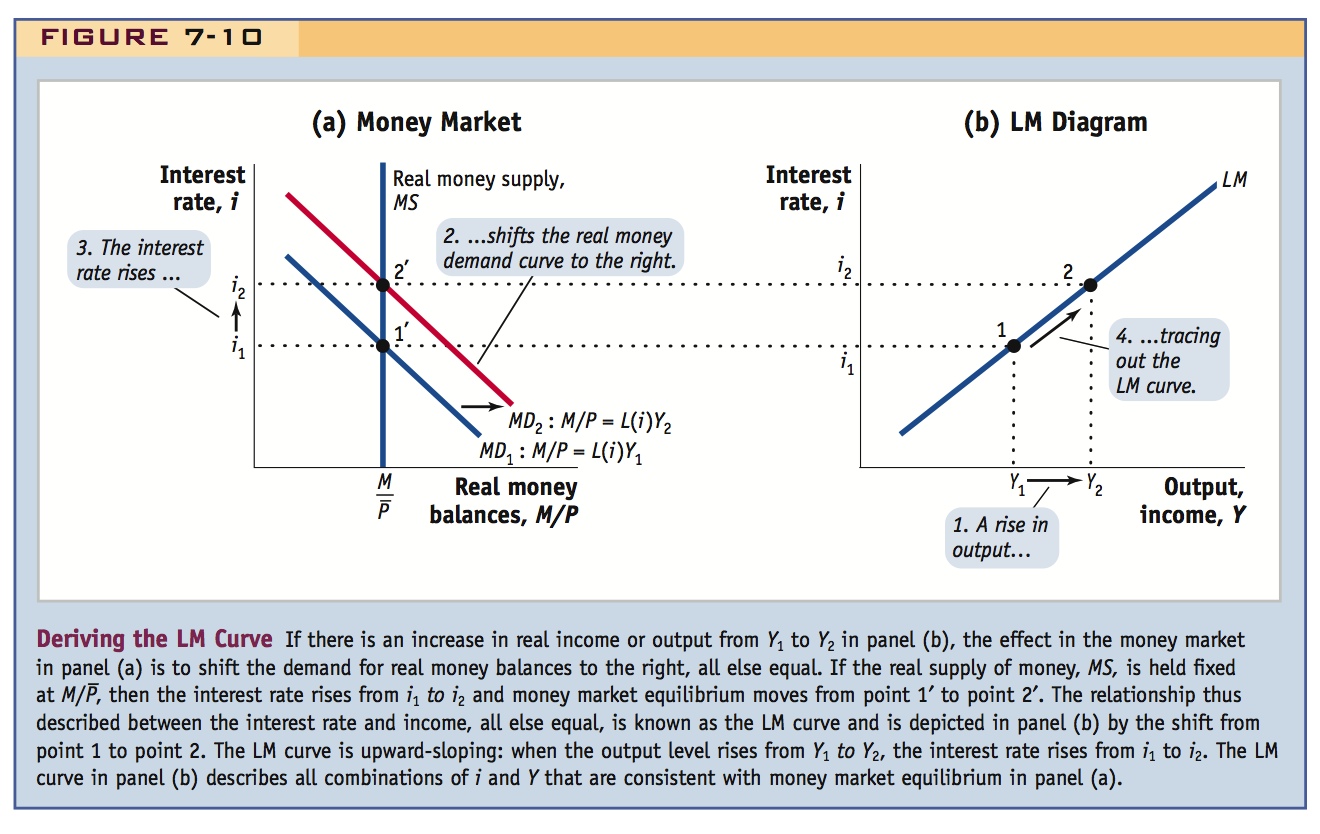
The LM curve shows combinations of Y and i such that the money market is in equilibrium. It is positively sloped because raising Y increases money demand, which increases i.
3. Factors that Shift the LM Curve
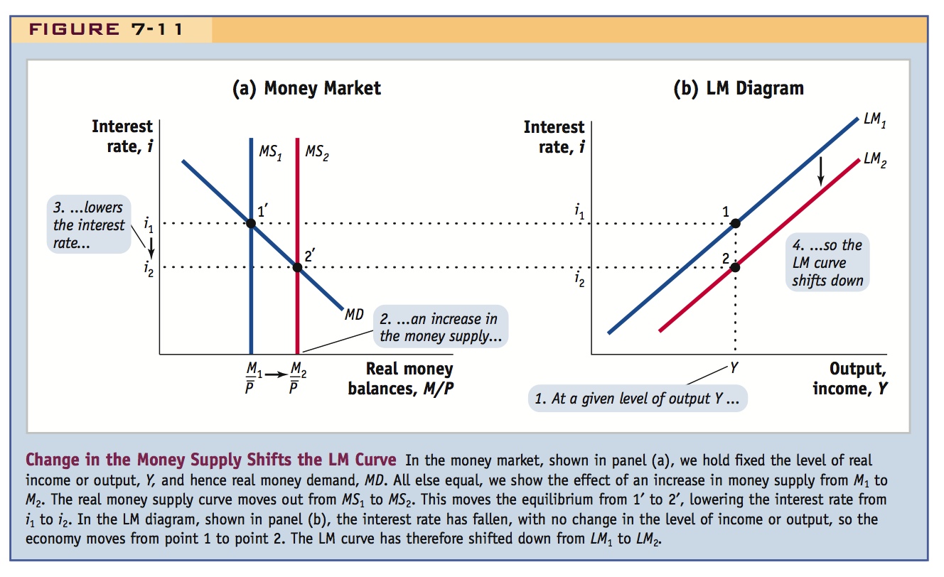
LM shifts to the right if M increases, Pdecreases, or if there is an exogenous fall in money demand.
4. Summing Up the LM Curve
The LM depicts equilibrium in the money market. It is positively sloped because income growth raises money demand. It will shift to the right if the money supply increases, prices fall, or there is an exogenous fall in money demand.
The IS curve links the forex market and the goods market as depicted by the Keynesian cross. It summarizes combinations of Y and i at which goods demand equals goods supply in a way that is consistent with forex market equilibrium. We have now taken care of equilibria in two out of three markets, so there is only one market left to worry about. In this section, we derive a set of combinations of Y and i that ensures equilibrium in the money market, a concept that can be represented graphically as the LM curve.
Say there is nothing new here, compared to their other macro classes
The LM curve is more straightforward to derive than the IS curve for a couple of reasons. First, the money market is something we have already studied in earlier chapters, so we already have all the tools we need to build the LM curve. Second, unlike the IS curve, the open-economy LM curve is no different from the closed-economy LM curve, so there will be no new material here if you have previously studied the closed-economy IS-LM model in another course.
Money Market Recap
In our earlier study of the money market, we assumed that the level of output or income Y was given. In deriving the LM curve, we now face a new question: What happens in the money market when an economy’s output changes?
In the short-run, the price level is assumed to be sticky at a level  , and the money market is in equilibrium when the demand for real money balances L(i)Y equals the real money supply
  :
:

Figure 7-10, panel (a), shows that real money demand MD varies inversely with the nominal interest rate. As a result of this relationship, the demand curve for real money balances slopes downward. The real money supply MS is assumed to be fixed for now. Initially, the level of output is at Y1 and the money market is in equilibrium at 1′, where real money demand is on MD1 at  .
.
If output changes, the real money demand curve shifts. For example, if output rises to Y2 and the real money supply  remains fixed, then real money demand increases because more output implies a larger number of transactions in the economy for which money is needed. The real money demand curve shifts right to MD2. To keep money supply and demand equal,
  , the interest rate rises from i = i1 to i = i2. Equilibrium moves from 1′ to 2′.
Deriving the LM Curve
This exercise can be repeated for any level of output Y. Doing so will generate a combination of interest rates i and outputs Y for which the money market is in equilibrium. This set of points, called the LM curve, is drawn in Figure 7-10, panel (b).

For example, if the real money supply is fixed at  , an increase in output from Y1 to Y2 generates a rise in the nominal interest rate from i1 to i2 in panel (a), as we have just seen. This change can also be depicted as a move from point 1 to point 2 along the LM curve, as shown in panel (b).
277
We have now derived the shape of the LM curve, which describes money market equilibrium. When output rises from Y1 to Y2, the interest rate rises from i1 to i2. The LM curve is an upward-sloping relationship between the interest rate i and output Y.
The two ways of depicting the money market equilibrium are entirely equivalent. The money market diagram shows the relationship between real money balances demanded and supplied at different interest rates, holding output fixed. The LM curve diagram shows the relationship between output and the interest rate holding real money balances as fixed. Because the LM curve does not hold output fixed, it is important to developing our model of how output, interest rates, and exchange rates fluctuate in the short run.
Factors That Shift the LM Curve
An important reason for a shift in the LM curve is a change in the real money supply. (Changes in output result in a move along a given LM curve.) The LM curve tells us the interest rate i that equilibrates the money market at any given level of output Y. Given Y, we know that the equilibrium interest rate i depends on real money supply  , and so the position of the LM curve depends on
  .
.
The effect of the real money supply on a nation’s output or income is important because we are often interested in the impact of monetary policy changes on overall economic activity. To see how this effect operates via the LM curve, we can examine the money market diagram in Figure 7-11, panel (a). An increase in the nominal money supply M with sticky prices raises real money supply from  to
to  and shifts the real money supply curve MS to the right.
278
What happens in the LM diagram if the exogenous real money supply  changes in this way? For a given level of output Y, the increased supply of real money drives the interest rate down to i2, and equilibrium in the money market shifts from point 1′ to point 2′. A decrease in the interest rate to i2 when the level of output is unchanged at Y means that we cannot be on the same LM curve as before. There must have been a downward shift of the LM curve from LM1 to LM2 in Figure 7-11, panel (b).

We have shown the following: an increase in real money supply shifts the LM curve down or to the right; a decrease in the real money supply shifts the LM curve up or to the left.
Thus, the position of the LM curve is a function of real money supply:

Remember that in this short-run model of the economy, prices are sticky and treated as given, so any change in the real money supply in the short run is caused by changes in the nominal money supply M, which for now we take as given or exogenous.
Use Y2K as an example, and ask how the Fed might have responded to keep interest rates constant.
This is another strategic place to introduce the liquidity trap. Have students figure out what LM looks like in that case, and how monetary policy affects it.
Other factors can influence the position of the LM curve. In addition to changes in the money supply, exogenous changes in real money demand will also cause the LM curve to shift. For example, for a given money supply, a decrease in the demand for real money balances (an increase in the L function) at a given level of output Y will tend to lower the interest rate, all else equal, which would be depicted as a shift down or to the right in the LM curve.
Summing Up the LM Curve
When prices are sticky, the LM curve summarizes the relationship between output Y and interest rate i necessary to keep the money market in short-run equilibrium for a given level of the real money supply. The LM curve is upward-sloping. Why? In a money market equilibrium, if real money supply is constant, then real money demand must also be constant. If output rises, real money demand rises and to maintain equilibrium, real money demand must contract. This contraction in real money demand is accomplished by a rise in the interest rate. Thus, on the LM curve, when output rises, so, too, does the interest rate.
279
The following factors shift the LM curve:

The opposite changes lead to an increase in the home interest rate and shift the LM curve up or to the left.