6 Stabilization Policy
Emphasize that Keynesian stabilization policies are only intended for short run, temporary shocks.
Stabilization policy attempts to use monetary or fiscal policies to keep the economy at full employment. However, it can backfire, if not used with care.
We now have seen that macroeconomic policies can effect economic activity in the short run. These effects open up the possibility that the authorities can use changes in policies to try to keep the economy at or near its full-employment level of output. This is the essence of stabilization policy. If the economy is hit by a temporary adverse shock, policy makers could use expansionary monetary and fiscal policies to prevent a deep recession. Conversely, if the economy is pushed by a shock above its full employment level of output, contractionary policies could tame the boom.
Go through the full analysis of Y2K as an example.
For example, suppose a temporary adverse shock such as a sudden decline in investment, consumption, or export demand shifts the IS curve to the left. Or suppose an adverse shock such as a sudden increase in money demand suddenly moves the LM curve up. Either shock would cause home output to fall. In principle, the home policy makers could offset these shocks by using fiscal or monetary policy to shift either the IS curve or LM curve (or both) to cause an offsetting increase in output. When used judiciously, monetary and fiscal policies can thus be used to stabilize the economy and absorb shocks.
The policies must be used with care, however. If the economy is stable and growing, an additional temporary monetary or fiscal stimulus may cause an unsustainable boom that will, when the stimulus is withdrawn, turn into an undesirable bust. In their efforts to do good, policy makers must be careful not to destabilize the economy through the ill-timed, inappropriate, or excessive use of monetary and fiscal policies.
This is a wonderful example. Use it as an excuse to work through the graphical tools, and highlight the policy implications.
In the financial crisis of 2008, both Poland and Latvia were hit with adverse demand shocks (declines in C,I, and TB). But the policy responses were different. Poland had a flexible exchange rate, so there was a depreciation that helped raise demand. At the same time, the Polish government raised expenditures and implemented a strong monetary expansion. So, Poland escaped a recession. Latvia was pegged to euro, so the fall in demand was reinforced by a fall in the money supplied, required to maintain the fixed rate. At the same time, Latvia implemented austerity policies by reducing government expenditures. Latvia fell into a deep recession.
The Right Time for Austerity?
After the global financial crisis, many observers would have predicted economic difficulties for Eastern Europe in the short run. Most countries had seen a rapid boom before 2008, with large expansions of credit, capital inflows, and high inflation of local wages and prices creating real appreciations: the same ingredients for a sharp economic downturn after the crisis as seen in Greece, Spain, Portugal and Ireland. Yet not all countries suffered the same fate. Here we use our analytical tools to look at two opposite cases: Poland, which fared well, and Latvia, which did not.
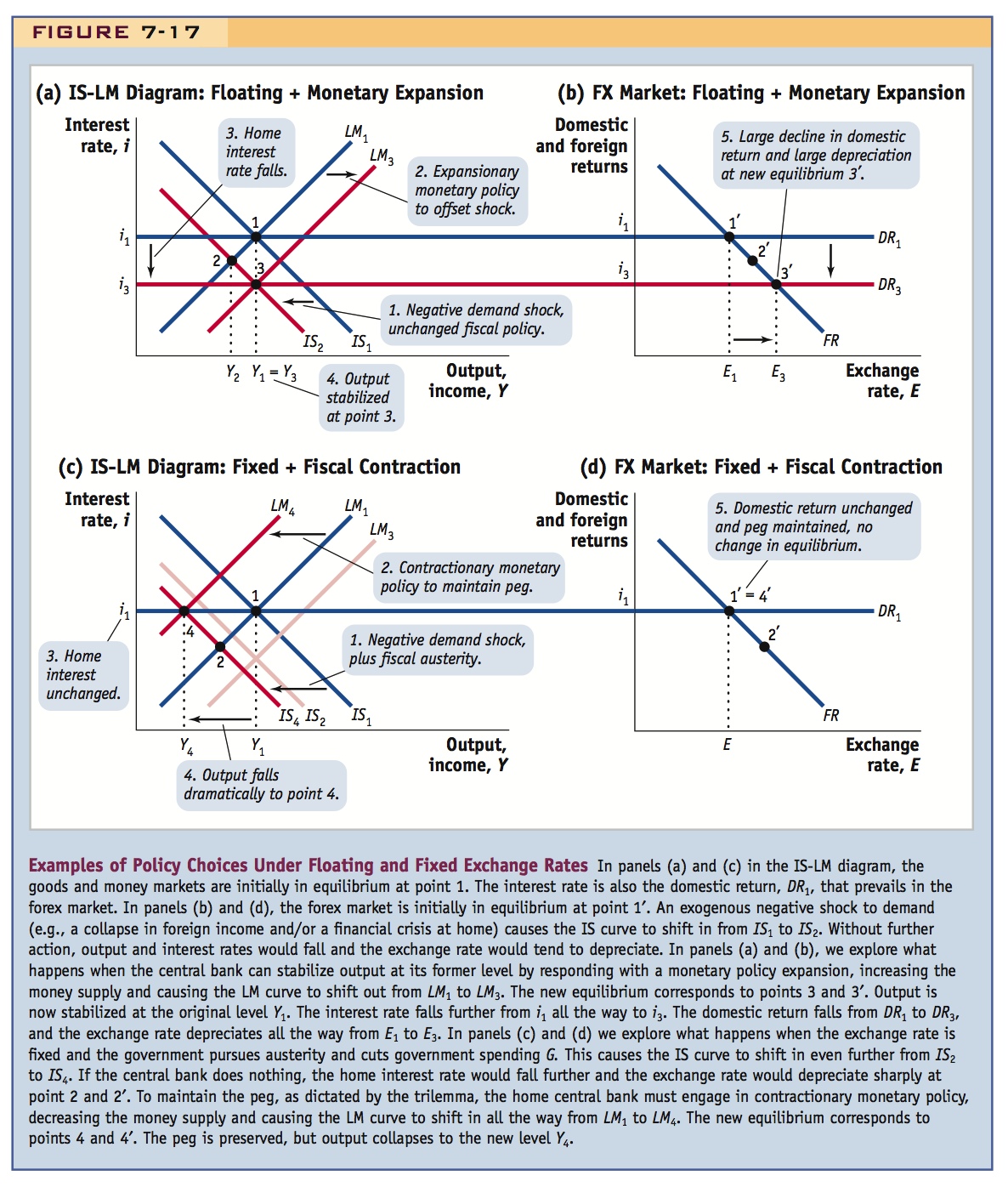
In our framework, as the shocks first hit, the demand for Poland’s and Latvia’s exports declined as a result of a contraction in foreign output Y* in their trading partners, mainly the rest of Europe. In addition Poland and Latvia faced negative shocks to consumption and investment demand as consumers and investors cut back their expenditures in the face of uncertainty and tighter credit due to financial sector problems. These events would be represented by a leftward shift of Poland’s and Latvia’s IS curves from IS1 to IS2, which we show in Figure 7-17.
But the policy responses differed in each country, illustrating the contrasts between fixed and floating regimes. Because the Poles had a floating exchange rate, they were able to pursue strong monetary expansion and let the currency depreciate. They also maintained their plans for government spending in order to combat the decline in demand. Because the Letts were pegging to the euro, they could not use monetary policy at all, and they had to pursue aggressive austerity and slash government spending in order to satisfy the demands of an EU and IMF assistance program. Our modeling framework makes some predictions about the consequences of these policy choices.
In Figure 7-17, panels (a) and (b), Poland first goes from points 1(1′) to point 2(2′), and the initial shock is partially offset by the induced depreciation of the Polish zloty and increased investment thanks to lower interest rates. Then the equilibrium would be at 2′. In the end, demand would still be below its initial level and a recession would result with output falling from Y1 to Y2. However, the central bank responded with expansionary monetary policy, a shift out in the LM curve to LM3. The economy shifted to point 3(3′): even lower interest rates amplified the depreciation of the zloty and stimulated demand through investment and expenditure-switching channels. In contrast, as shown in Figure 7-17, panels (c) and (d), Latvia cut government spending, so when their IS curve shifted in, they shifted it even farther to IS4. Bound by the trilemma, Latvia’s LM curve had to follow those shifts in lockstep and move in to LM4 in order to maintain the lat–euro peg. The Latvian economy moved from point 1(1′) to point 4(4′).
288
289
The model predicts that a recession might be avoided in Poland, but that there could be a very deep recession in Latvia. What actually happened? Check out the accompanying news item (see Headlines: Poland Is Not Latvia).
Problems in Policy Design and Implementation
In this chapter, we have looked at open-economy macroeconomics in the short run and at the role that monetary and fiscal policies can play in determining economic outcomes. The simple models we used have clear consequences. On the face of it, if policy makers were really operating in such an uncomplicated environment, they would have the ability to exert substantial control and could always keep output steady with no unemployed resources and no inflation pressure. In reality, life is more complicated for policy makers for a variety of reasons.
Students often think stabilization policy is as simple as shifting the curves around, so it is important to remind them of all of these constraints.
Policy Constraints Policy makers may not always be free to apply the policies they desire. A fixed exchange rate rules out any use of monetary policy. Other firm monetary or fiscal policy rules, such as interest rate rules or balanced-budget rules, place limits on policy. Even if policy makers decide to act, other constraints may bind them. While it is always feasible to print money, it may not be possible (technically or politically) to raise the real resources necessary for a fiscal expansion. Countries with weak tax systems or poor creditworthiness—problems that afflict developing countries—may find themselves unable to tax or borrow to finance an expansion of spending even if they wished to do so.
But argue monetary policy is much faster, even overnight. Ask them how long they think it takes Congress to pass an appropriations bill? Point out that fiscal policy could even be destabilizing if it takes too long to get in place.
Incomplete Information and the Inside Lag Our models assume that the policy makers have full knowledge of the state of the economy before they take corrective action: they observe the economy’s IS and LM curves and know what shocks have hit. In reality, macroeconomic data are compiled slowly and it may take weeks or months for policy makers to fully understand the state of the economy today. Even then, it will take time to formulate a policy response (the lag between shock and policy actions is called the inside lag). On the monetary side, there may be a delay between policy meetings. On the fiscal side, it may take even more time to pass a bill through the legislature and then enable a real change in spending or taxing activity by the public sector.
This is Friedman's taxonomy of lags.
Policy Response and the Outside Lag Even if they finally receive the correct information, policy makers then have to formulate the right response given by the model. In particular, they must not be distracted by other policies or agendas, nor subject to influence by interest groups that might wish to see different policies enacted. Finally, it takes time for whatever policies are enacted to have any effect on the economy, through the spending decisions of the public and private sectors (the lag between policy actions and effects is called the outside lag).
Long-Horizon Plans Other factors may make investment and the trade balance less sensitive to policy. If the private sector understands that a policy change is temporary, then there may be reasons not to change consumption or investment expenditure.
290
An article commenting on how much worse Latvia fared than Poland.
1. Problems in Policy Design and Implementation
Our analysis might suggest that it is easy to implement stabilization policies. In fact, it is quite difficult, for a variety of reasons:
a. Policy Constraints
Fixed rates preclude the use of monetary policy. Interest rate rules or balanced budget rules may also limit policy responses. Excessive money growth may cause inflation; excessive borrowing may weaken access to credit.
b. Incomplete Information and the Inside Lag
Macro data is unreliable and collected with lags, so the government does not know exactly where the IS and LM curves are at a given time. It also takes time to formulate a response (the “inside” lag).
c. Policy Response and the Outside Lag
Once they have decided upon a policy, policymakers must stick to it, and not be distracted by other objectives. Furthermore, it takes time for the policy to take effect, once it is implemented (the “outside” lag).
d. Long-Horizon Plans
Consumers and firms may not respond strongly to policy changes if they anticipate that they will be temporary.
e. Weak Links from the Nominal Exchange Rate to the Real Exchange Rate
Nominal depreciation may not result in real depreciation if there is weak pass-through. This could be caused by dollarization or pricing to market.
f. Pegged Currency Blocs
If a large bloc of countries is pegged to the dollar, it is hard for the U.S. to implement a depreciation of its effective exchange rate.
g. Weak Links from the Real Exchange Rate to the Trade Balance
Because of transaction costs, the effect of a depreciation on may be weak at first, but get stronger as the depreciation increases. Combined with the J Curve, this implies that a depreciation may not initially affect the much, or even push it in the wrong direction.
Poland Is Not Latvia
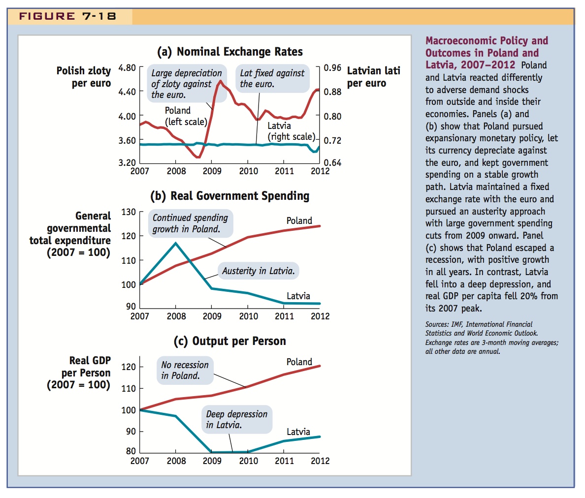
Eastern Europe faced difficult times in the Great Recession. Yet not all countries suffered the same fate, as we see from this story, and the macroeconomic data presented and discussed in Figure 7-18.
…Poland and Latvia…inherited woefully deficient institutions from communism and have struggled with many of the same economic ills over the past two decades. They have also adopted staggeringly different approaches to the crisis, one of which was a lot more effective than the other.
…I don’t think it’s being radical to say that [since 2004] Poland’s performance is both a lot better and a lot less variable and that if you were going to draw lessons from one of the two countries that it should probably be the country which avoided an enormous bubble and subsequent collapse. What is it that caused Poland’s economy to be so sound? Was it austerity? Was it hard money?
…Both Latvia and Poland actually ran rather substantial budget deficits during the height of the crisis, though Latvia’s budgeting in the years preceding the crisis was more balanced and restrained than Poland’s…. Poland’s government spending as a percentage of GDP was also noticeably higher than Latvia’s both before the crisis and after it…. You can see how, starting in 2008, Latvia starts to make some sharp cuts while Poland continues its steady, modest increases.
291
So, basically, Poland is a country whose government habitually ran budget deficits before, during, and after the crisis, whose government spends a greater percentage of GDP than Latvia, and which did not cut spending in response to the crisis. Latvia, in contrast, ran balanced budgets, had a very small government as a percentage of GDP, and savagely cut spending in response to the crisis. While I don’t think you can call Poland “profligate,” if economics really were a morality play you’d expect the Latvians to come out way ahead since they’ve followed the austerity playbook down to the letter. However, in the real world, Poland’s economic performance has been vastly, almost comically, superior to Latvia’s despite the fact that the country didn’t make any “hard choices.”
All of this, of course, leaves out monetary policy…. Part of the reason that Latvia’s economic performance has been so awful is that it has pegged its currency to the Euro, a course of action which has made the Lat artificially expensive and which made Latvia’s course of “internal devaluation” necessary…. Poland did the exact opposite, allowing its currency, the zloty, to depreciate massively against the Euro …
Poland did not, in other words, “defend the zloty” because it realized that a devaluation of its currency would be incredibly helpful. And the Polish economy has continued to churn along while most of its neighbors have either crashed and burned or simply stagnated….
There are plenty of lessons from Poland’s economic success, including the need for effective government regulation (Poland never had an out-of-control bubble like Latvia), the need for exchange rate flexibility, and the extreme importance of a country having its own central bank. These lessons are neither left wing nor right wing, Poland’s government is actually quite conservative…Economics just isn’t a morality play, and no matter how often the Latvians cast themselves as the diligent and upstanding enforcers of austerity their economic performance over the past five years has still been lousy.
Source: Excerpted from Mark Adomanis, “If Austerity Is So Awesome Why Hasn’t Poland Tried It?” forbes.com, January 10, 2013. Reproduced with Permission of Forbes Media LLC © 2013.
Suppose a firm can either build and operate a plant for several years or not build at all (e.g., the investment might be of an irreversible form). For example, a firm may not care about a higher real interest rate this year and may base its decision on the expected real interest rate that will affect its financing over many years ahead. Similarly, a temporary real appreciation may have little effect on whether a firm can profit in the long run from sales in the foreign market. In such circumstances, firms’ investment and export activities may not be very sensitive to short-run policy changes.
Weak Links from the Nominal Exchange Rate to the Real Exchange Rate Our discussion assumed that changes in the nominal exchange rate lead to real exchange rate changes, but the reality can be somewhat different for some goods and services. For example, the dollar depreciated 42% against the yen from 2008 to 2012, but the U.S. prices of Japanese-made cars, like some Toyotas, barely changed. Why? There are a number of reasons for this weak pass-through phenomenon, including the dollarization of trade and the distribution margins that separate retail prices from port prices (as we saw in Side Bar: Barriers to Expenditure Switching: Pass-Through and the J Curve). The forces of arbitrage may also be weak as a result of noncompetitive market structures: for example, Toyota sells through exclusive dealers and government regulation requires that cars meet different standards in Europe versus the United States. These obstacles allow a firm like Toyota to price to market: to charge a steady U.S. price even as the exchange rate moves temporarily. If a firm can bear (or hedge) the exchange rate risk, it might do this to avoid the volatile sales and alienated customers that might result from repeatedly changing its U.S. retail price list.
Pegged Currency Blocs Our model’s predictions are also affected by the fact that for some major countries in the real world, their exchange rate arrangements are characterized—often not as a result of their own choice—by a mix of floating and fixed exchange rate systems with different trading partners. For most of the decade 2000–10, the dollar depreciated markedly against the euro, pound, and several other floating currencies, but in the emerging-market “Dollar Bloc” (China, India, and other countries), the monetary authorities have ensured that the variation in the value of their currencies against the dollar was small or zero. When a large bloc of other countries pegs to the U.S. dollar, this limits the ability of the United States to engineer a real effective depreciation.
292
Weak Links from the Real Exchange Rate to the Trade Balance Our discussion also assumed that real exchange rate changes lead to changes in the trade balance. There may be several reasons why these linkages are weak in reality. One major reason is transaction costs in trade. Suppose the exchange rate is $1 per euro and an American is consuming a domestic good that costs $100 as opposed to a European good costing €100 = $100. If the dollar appreciates to $0.95 per euro, then the European good looks cheaper on paper, only $95. Should the American switch to the import? Yes, if the good can be moved without cost—but there are few such goods! If shipping costs $10, it still makes sense to consume the domestic good until the exchange rate falls below $0.90 per euro. Practically, this means that expenditure switching may be a nonlinear phenomenon: it will be weak at first and then much stronger as the real exchange rate change grows larger. This phenomenon, coupled with the J curve effects discussed earlier, may cause the response of the trade balance in the short run to be small or even in the wrong direction.
In a liquidity trap—also known as the zero-lower bound (ZLB)—the LM curve is horizontal at very low interest rates. In this case conventional monetary policy is ineffective, but fiscal policy is very strong. The U.S. tried to use expansionary fiscal policy during the Great Recession: (1) automatic stabilizers kicked in, and the stimulus bill was implemented. Many economists thought the stimulus package was too small. Other things limited its effectiveness. First, tax cuts had little effect on consumption. Some people were uncertain about the future and saved more; others may have anticipated future tax increases, and so saved more (the Ricardian view). Second, although federal spending increased, state and local spending decreased by about the same amount. The net fiscal stimulus was about zero. So monetary policy was impotent, and the fiscal response was too small and ill-designed.
This is a great example, but enrich it by arguing perhaps that I became less interest elastic, so IS got steeper. In this case fiscal policy should have been even more effective. Also use this as an opportunity to discuss QE and forward guidance as an alternative to the conventional monetary policy.
Macroeconomic Policies in the Liquidity Trap
Undoubtedly, one of the most controversial experiments in macroeconomic policy-making began in 2008–10 as monetary and fiscal authorities around the world tried to respond to the major recession that followed the Global Financial Crisis. In this application, we look at the initial U.S. policy response and interpret events using the IS-LM-FX model of this chapter.
The unusual aspect of this crisis was the very rapid realization that monetary policy alone could not fully offset the magnitude of the shock to demand. In the context of our IS-LM-FX model, as consumption and investment fell for exogenous reasons, the shock moved the IS curve very far leftward. One major source of the demand shock was that, as we saw in an earlier chapter, banks were very afraid of taking on risk and sharply reduced their lending to firms and households—and even when they did lend, they were still charging very high interest rates. Thus, even with very expansionary monetary policy, that is, large rightward shifts of the LM curve, low policy interest rates did not translate into cheap borrowing for the private sector. Once the U.S. Federal Reserve had brought its policy rate to zero in December 2008, there was little more it could do to stimulate demand using conventional monetary policies.
This peculiar situation is depicted by the blue lines in Figure 7-19 and differs from the normal IS-LM-FX setup we have seen so far. After the demand shock and the Fed’s response to it, the IS curve has moved so far in (to IS1) and the LM curve has moved so far out (to LM1), that the IS and LM curves now intersect at a very low interest rate: so low that it is equal to zero. In the money market, nominal interest rates can’t fall below zero, so another way of describing this situation is to say that the economy was at an IS-LM equilibrium at which the LM curve was absolutely flat and resting on the horizontal axis (at a 0% interest rate) in the diagram.
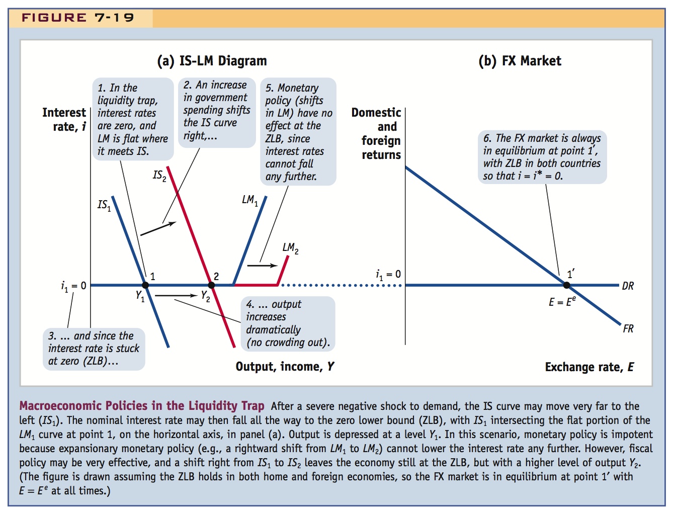
(Note that in the FX diagram this would place the domestic return DR at zero. Also, note that interest rates were by this time at zero in all developed countries, for similar reasons. Thus, it is also appropriate to think of the foreign (e.g., euro) interest rate as also stuck at zero, which in the FX diagram would lower the foreign return FR.)
293
The situation just described is unusual in several ways. First, monetary policy is powerless in this situation: it cannot be used to lower interest rates because interest rates can’t go any lower. In the diagram, moving the LM curve out to LM2 does not dislodge the economy from the horizontal portion of the LM curve. We are still stuck on the IS1 curve at a point 1 and a 0% percent interest rate. This unfortunate state of affairs is known as the zero lower bound (ZLB). It is also known as a liquidity trap because liquid money and interest-bearing assets have the same interest rate of zero, so there is no opportunity cost to holding money, and thus changes in the supply of central bank money have no effect on the incentive to switch between money and interest-bearing assets.
Can anything be done? Yes. The bad news is that fiscal policy is the only tool now available to increase demand. The good news is that fiscal policy has the potential to be super powerful in this situation. The reason is that as long as interest rates are stuck at zero, and the monetary authorities keep them there, government spending will not crowd out investment or net exports, in contrast to the typical situation we studied earlier in this chapter.3 In 2009, because the Fed and the private sector anticipated more than a year or two of very high unemployment and falling inflation, everyone had expectations of zero interest rates for a long period.
294
Did the United States use fiscal policy to try to counteract the recession? Yes. Did it work? Not as well as one might have hoped.
The government’s fiscal response took two forms. First was the automatic stabilizer built into existing fiscal policies. In the models that we have studied so far in this chapter, we have assumed that taxes and spending are fixed. In reality, however, they are not fixed, but vary systematically with income. Most important, when income Y falls in a recession, receipts from income taxes, sales taxes, and so on, all tend to fall as well. In addition, transfer expenditures (like unemployment benefits) tend to go up: a rise in negative taxes, as it were. This decline does not depend on any policy response, and in the 2008–10 period the fall in tax revenues (plus the rise in transfers) was enormous.
The second fiscal response was a discretionary policy, the American Recovery and Reinvestment Act (ARRA), better known as the “stimulus” bill. This policy was one of the first actions undertaken by the Obama administration and it was signed into law on February 17, 2009. Some of the president’s advisors had originally hoped for a $1.4 trillion package, mostly for extra government consumption and investment spending, and also for aid to states. This was to be spread over 2 to 3 years from 2009–11. However, the final compromise deal with Congress was only half as big, $787 billion over three years, and was tilted more toward temporary tax cuts. Most of the stimulus was scheduled to take effect in 2010, not 2009, reflecting the policy lags we noted above. On average, the package amounted to about 1.5% of GDP in spending and tax cuts.
Some key outcomes are shown in Figure 7-20. As panel (a) shows, the size of the gap between actual and potential output left a huge hole to be filled by fiscal policy. By mid-2009 this hole was about 6% of potential GDP or over $1 trillion at an annual rate. Even if the entire stimulus were spent, the fiscal package could at best have filled only about one-quarter of the collapse in demand or 1.5% of GDP. Policy makers in the government, and many observers, knew the package was too small, but politics stood in the way of a larger package.
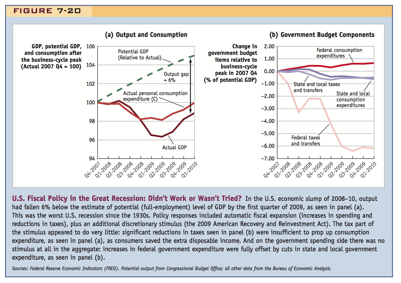

The data in panel (a) also show that private consumption fell precipitously. One intention of ARRA was to support private spending through tax cuts. Tax revenues T did fall considerably (largely at the federal level as shown in panel (b), because states were getting some offsetting transfers via ARRA). But tax cuts did not appear to generate much extra private spending, certainly not enough to offset the initial collapse in consumption expenditure. Many consumers were unsure about the economic recovery, worried about the risks of unemployment, and trying to use whatever “extra” money they got from tax cuts to pay down their debts or save. In addition, because people were trying to hold onto their money (precautionary motives were high), the marginal propensity to consume was probably low. Furthermore, for non-Keynesian consumers, the temporary nature of many of the tax cuts meant that anyone following the principles of Ricardian equivalence would be likely to save the tax cut to pay off an expected future tax liability.
This left government spending G to do a great deal of the stimulation, but problems arose because of the contrary effects of state and local government policies. As the figure shows, federal expenditures went up, rising by 0.5% of GDP in 2010. Leaving aside the miniscule size of this change, a big source of trouble was that state and local government expenditures went down by just as much. States and localities imposed austerity spending cuts, which were made necessary by calamitous declines in their tax revenues, by their limited ability (or willingness) to borrow, and by the feeble amount of aid to states authorized in the final ARRA package. The net change in overall government expenditures was thus, in the end, zero.
295
To sum up, the aggregate U.S. fiscal stimulus had four major weaknesses: it was rolled out too slowly, because of policy lags; the overall package was too small, given the magnitude of the decline in aggregate demand; the government spending portion of the stimulus, for which positive expenditure effects were certain, ended up being close to zero, because of state and local cuts; and this left almost all the work to tax cuts (automatic and discretionary) that recipients, for good reasons, were more likely to save rather than spend. With monetary policy impotent and fiscal policy weak and ill designed, the economy remained mired in its worst slump since the 1930s Great Depression.4
It would be useful to talk about tax cuts as a separate comparative static exercise earlier, distinguishing between the conventional and Ricardian interpretations.
This is an excellent summary.
296