3 Determining the Pattern of International Trade
1. Objective: Explain why countries trade, and predict which goods they will export and import.
2. International Trade Equilibrium
a.Intuitive argument:
i. Allow trade. (Relative) Price of wheat is higher abroad than it is at home, so Home would like to sell its wheat to foreigners. Conversely, Foreign would like to sell its cloth to Home.
ii. Therefore, there are mutually beneficial gains from trade.
iii. Trade causes relative prices to be the same in both counties.
b. Change in Production and Consumption
Expansion of the wheat industry raises wages there. All workers go to the wheat sector.
c. International Trade
i.Home specializes in wheat and exports it at a price above its opportunity cost. Consumption possibilities have increased, so home enjoys gains from trade.
ii.Repeat argument for Foreign.
iii.Conclusions:
(1)Each country will export the good for which it has a comparative advantage.
(2)Both countries gain from trade.
d. Solving for Wages Across Countries
Prices of goods equalize with trade, but wages do not: Real wages—regardless of whether they are measured in cloth or wheat—depend upon marginal productivity in the export sectors.
e. Absolute Advantage
Frequently overlooked conclusion of the Ricardian model: Real wages are determined by absolute productivity.
Now that we have examined each country in the absence of trade, we can start to analyze what happens when goods are traded between them. We will see that a country’s no-trade relative price determines which product it will export and which it will import when trade is opened. Earlier, we saw that the no-trade relative price in each country equals its opportunity cost of producing that good. Therefore, the pattern of exports and imports is determined by the opportunity costs of production in each country, or by each country’s pattern of comparative advantage. This section examines why this is the case and details each country’s choice of how much to produce, consume, and trade of each good.
41
International Trade Equilibrium
Emphasize that trade is caused by differences in autarky prices.
Again, if you've called the opportunity cost of wheat the "MC" of wheat in terms of cloth, then with trade P > MC for wheat. Students can apply their micro intuition to see that Home should produce as much wheat as it can.
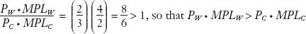
The differences in no-trade prices across the countries create an opportunity for international trade between them. In particular, producers of cloth in Foreign, where the relative price of cloth is  = 1, would want to export cloth to Home, where the relative price, PC/PW = 2, is higher. Conversely, producers of wheat in Home, where the relative price of wheat is PW/PC =
  , would want to export wheat to Foreign, where the relative price of
  = 1 is higher. The trade pattern that we expect to arise, then, is that Home will export wheat, and Foreign will export cloth. Notice that both countries export the good in which they have a comparative advantage, which is what the Ricardian model predicts.
To solidify our understanding of this trade pattern, let’s be more careful about explaining where the two countries would produce on their PPFs under international trade and where they would consume. As Home exports wheat, the quantity of wheat sold at Home falls, and this condition bids up the price of wheat in the Home market. As the exported wheat arrives in the Foreign wheat market, more wheat is sold there, and the price of wheat in the Foreign market falls. Likewise, as Foreign exports cloth, the price of cloth in Foreign will be bid up and the price of cloth in Home will fall. The two countries are in an international trade equilibrium, or just “trade equilibrium,” for short, when the relative price of wheat is the same in the two countries, which means that the relative price of cloth is also the same in both countries.8
To fully understand the international trade equilibrium, we are interested in two issues: (1) determining the relative price of wheat (or cloth) in the trade equilibrium and (2) seeing how the shift from the no-trade equilibrium to the trade equilibrium affects production and consumption in both Home and Foreign. Addressing the first issue requires some additional graphs, so let’s delay this discussion for a moment and suppose for now that the relative price of wheat in the trade equilibrium is established at a level between the pre-trade prices in the two countries. This assumption is consistent with the bidding up of export prices and bidding down of import prices, as discussed previously. Since the no-trade prices were PW/PC = in Home and = 1 in Foreign, let’s suppose that the world relative price of wheat is between these two values, say, at  . Given the change in relative prices from their pre-trade level to the international trade equilibrium, what happens to production and consumption in each of the two countries?
8 Notice that if the relative price of wheat PW/PC is the same in the two countries, then the relative price of cloth, which is just its inverse (PC/PW), is also the same.
Change in Production and Consumption The world relative price of wheat that we have assumed is higher than Home’s pre-trade price ( > ). This relationship between the pre-trade and world relative prices means that Home producers of wheat can earn more than the opportunity cost of wheat (which is 1/2) by selling their wheat to Foreign. For this reason, Home will shift its labor resources toward the production of wheat and produce more wheat than it did in the pre-trade equilibrium (point A in Figure 2-5). To check that this intuition is correct, let us explore the incentives for labor to work in each of Home’s industries.

42
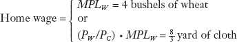
Recall that Home wages paid in the wheat industry equal PW · MPLW, and wages paid in the cloth industry equal PC · MPLC. We know that the relative price of wheat in the trade equilibrium is PW/PC = , that the marginal product of labor in the Home wheat industry is MPLW = 4, and that the marginal product of labor in the Home cloth industry is MPLC = 2. We can plug these numbers into the formulas for wages to compute the ratio of wages in the two industries as
This formula tells us that with the world relative price of wheat, wages paid in Home’s wheat industry (PW · MPLW) are greater than those paid in its cloth industry (PC · MPLC). Accordingly, all of Home’s workers will want to work in the wheat industry, and no cloth will be produced. With trade, the Home economy will be fully specialized in wheat production, as occurs at production point B in Figure 2-5.9
9 The fully specialized economy (producing only wheat) is a special feature of the Ricardian model because of its straight-line production possibilities frontier.
43
Here it may be useful to derive the budget constraint algebraically, emphasizing that the autarky budget constraint is coincident with the PPF, but that trade rotates the budget constraint outside the trade.
International Trade Starting at the production point B, Home can export wheat at a relative price of . This means that for 1 bushel of wheat exported to Foreign, it receives yard of cloth in exchange. In Figure 2-5, we can trace out its international trades by starting at point B and then exchanging 1 bushel of wheat for yard of cloth, another bushel of wheat for yard of cloth, and so on. From point B, this traces out the line toward point C, with slope −. We will call the line starting at point B (the production point) and with a slope equal to the negative of the world relative price of wheat, the world price line, as shown by BC. The world price line shows the range of consumption possibilities that a country can achieve by specializing in one good (wheat, in Home’s case) and engaging in international trade (exporting wheat and importing cloth). We can think of the world price line as a new budget constraint for the country under international trade.
Do another example of where consumption of both goods increases with trade. Emphasize that the gains from trade do not depend upon consumption of both goods increasing, that the gains from trade arise from the enlargement of the consumption opportunities set.
Notice that this budget constraint (the line BC) lies above Home’s original PPF. The ability to engage in international trade creates consumption possibilities for Home that were not available in the absence of trade, when the consumption point had to be on Home’s PPF. Now, Home can choose to consume at any point on the world price line, and utility is maximized at the point corresponding to the intersection with highest indifference curve, labeled C with a utility of U2. Home obtains a higher utility with international trade than in the absence of international trade (U2 is higher than U1); the finding that Home’s utility increases with trade is our first demonstration of the gains from trade, by which we mean the ability of a country to obtain higher utility for its citizens under free trade than with no trade.
Pattern of Trade and Gains from Trade Comparing production point B with consumption point C, we see that Home is exporting 100 − 40 = 60 bushels of wheat, in exchange for 40 yards of cloth imported from Foreign. If we value the wheat at its international price of , then the value of the exported wheat is · 60 = 40 yards of cloth, and the value of the imported cloth is also 40 yards of cloth. Because Home’s exports equal its imports, this outcome shows that Home’s trade is balanced.
What happens in Foreign when trade occurs? Foreign’s production and consumption points are shown in Figure 2-6. The world relative price of wheat () is less than Foreign’s pre-trade relative price of wheat (which is 1). This difference in relative prices causes workers to leave wheat production and move into the cloth industry. Foreign specializes in cloth production at point B*, and from there, trades along the world price line with a slope of (negative) , which is the relative price of wheat. That is, Foreign exchanges yard of cloth for 1 bushel of wheat, then yard of cloth for another 1 bushel of wheat, and so on repeatedly, as it moves down the world price line B*C*. The consumption point that maximizes Foreign’s utility is C*, at which point 60 units of each good are consumed and utility is  . Foreign’s utility is greater than it was in the absence of international trade ( is a higher indifference curve than
  ), as is true for Home. Therefore, both countries gain from trade.

44
Emphasize these italicized lines.
Foreign produces 100 yards of cloth at point B*: it consumes 60 yards itself and exports 100 −60 = 40 yards of cloth in exchange for 60 bushels of wheat imported from Home. This trade pattern is exactly the opposite of Home’s, as must be the case. In our two-country world, everything leaving one country must arrive in the other. We see that Home is exporting wheat, in which it has a comparative advantage (Home’s opportunity cost of wheat production is yard of cloth compared with 1 yard in Foreign). Furthermore, Foreign is exporting cloth, in which it has a comparative advantage (Foreign’s opportunity cost of cloth production is 1 bushel of wheat compared with 2 bushels in Home). This outcome confirms that the pattern of trade is determined by comparative advantage, which is the first lesson of the Ricardian model. We have also established that there are gains from trade for both countries, which is the second lesson.
These two conclusions are often where the Ricardian model stops in its analysis of trade between countries, but the story is incomplete because we have not yet determined the level of wages across countries. We have seen that with trade, the relative price of each good converges to a single equilibrium price in both countries. Does the same occur with wages? As we now show, this is not the case. Wage levels differ across countries with trade, and wages are determined by absolute advantage, not comparative advantage. This is a third, less emphasized lesson from the Ricardian model, which we explore next.
45
Solving for Wages Across Countries To understand how wages are determined, we go back to microeconomics. In competitive labor markets, firms will pay workers the value of their marginal product. Home produces and exports wheat, so we can think of Home workers being paid in terms of that good: their real wage is MPLW = 4 bushels of wheat. We refer to this payment as a “real” wage because it is measured in terms of a good that workers consume and not in terms of money. The workers can then sell the wheat they earn on the world market at the relative price of PW/PC = . Thus, their real wage in terms of units of cloth is (PW/PC) · MPLW = · 4 =  yard. Summing up, the Home wage is10
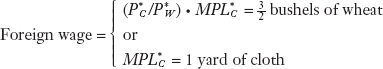
What happens to Foreign wages? Foreign produces and exports cloth, and the real wage is  = 1 yard of cloth. Because cloth workers can sell the cloth they earn for wheat on the world market at the price of
  , their real wage in terms of units of wheat is () · = · 1 = bushel. Thus, the Foreign wage is11
Students will ask which way of measuring real wages is "correct." Explain that what matters is that real wages are always lower in the the country with the absolute disadvantage, REGARDLESS of how real wages are measured.
Foreign workers earn less than Home workers as measured by their ability to purchase either good. This fact reflects Home’s absolute advantage in the production of both goods.
10 Recall that without international trade, Home wages were MPLW = 4 bushels of wheat or MPLC = 2 yards of cloth. Home workers are clearly better off with trade because they can afford to buy the same amount of wheat as before (4 bushels) but more cloth (yards instead of 2 yards). This is another way of demonstrating the gains from trade.
11 Without international trade, Foreign wages were MPL*W = 1 bushel of wheat or MPL*C = 1 yard of cloth. Foreign workers are also better off with trade because they can afford to buy the same amount of cloth (1 yard) but more wheat (bushels instead of 1 bushel).
Absolute Advantage As our example shows, wages are determined by absolute advantage: Home is paying higher wages because it has better technology in both goods. In contrast, the pattern of trade in the Ricardian model is determined by comparative advantage. Indeed, these two results go hand in hand—the only way that a country with poor technology can export at a price others are willing to pay is by having low wages.
This statement might sound like a pessimistic assessment of the ability of less developed countries to pay reasonable wages, but it carries with it a silver lining: as a country develops its technology, its wages will correspondingly rise. In the Ricardian model, a logical consequence of technological progress is that workers will become better off through receiving higher wages. In addition, as countries engage in international trade, the Ricardian model predicts that their real wages will rise.12 We do not have to look very hard to see examples of this outcome in the world. Per capita income in China in 1978, just as that nation began to open up to international trade, is estimated to have been $755 (all numbers are in 2005 dollars), whereas 32 years later in 2010, per capita income in China had risen by nearly 10 times to $7,437. Likewise for India, per capita income more than tripled from $1,040 in 1978 to $3,477 in 2010.13 Many people believe that the opportunity for these countries to engage in international trade has been crucial in raising their standard of living. As our study of international trade proceeds, we will try to identify the conditions that have allowed China, India, and many other developing countries to improve their standards of living through trade.
12 That result is shown by the comparison of real wages in the trade equilibrium as compared with the no-trade equilibrium in each country, as is done in the previous two footnotes.
13 These values are expressed in 2005 dollars and are taken from the Penn World Table version 7.1, http://pwt.econ.upenn.edu, averaging Version 1 and Version 2 for China.
46
Some students may ask why real wages in the U.S. have be stagnant if productivity has been increasing. Allude to the usual suspects (e.g. outsourcing, reduced demand for unskilled labor as productivity increases). But promise more on this will come.
Empirical data supporting the assertion that wages increase with productivity.
Labor Productivity and Wages
The close connection between wages and labor productivity is evident by looking at data across countries. Labor productivity can be measured by the value-added per hour in manufacturing. Value-added is the difference between sales revenue in an industry and the costs of intermediate inputs (e.g., the difference between the value of a car and the cost of all the parts used to build it). Value-added then equals the payments to labor and capital in an industry. In the Ricardian model, we ignore capital, so we can measure labor productivity as value-added divided by the number of hours worked, or value-added per hour.
In Figure 2-7, we show the value-added per hour in manufacturing in 2010 for several different countries. The United States has the highest level of productivity and Taiwan has the lowest for the countries shown. Figure 2-7 also shows the wages per hour paid in each country. These are somewhat less than value-added per hour because value-added is also used to pay capital. We see that the highest productivity countries shown—the United States and France—have higher wages than the lowest productivity countries shown—South Korea and Taiwan. But the middle countries—Italy, Japan, and Sweden—have wages at or above the U.S. level, despite having lower productivity. That is because the wage being used includes the benefits received by workers, in the form of medical benefits, Social Security, and so on. Many European countries and Japan have higher social benefits than the United States. Although including benefits distorts the comparison between wages and productivity, we still see from Figure 2-7 that higher productivity countries tend to have higher wages, broadly speaking, as the Ricardian model predicts. The connection between productivity and wages is also evident if we look at countries over time. Figure 2-8 shows that the general upward movement in labor productivity is matched by upward movement in wages, also as the Ricardian model predicts.


47