1 Specific-Factors Model
1. Objective:
Explain how trade affects the returns to land, labor, and capital.
Intuition: In the Ricardian model, trade raises wages by increasing the relative price of the export good. Similarly, here the basic question is how changes in relative prices of goods affect the returns to the factors. Specific factors are “stuck,” so their returns rise or fall with changes in goods’ prices in their sector; mobile factors are less affected, since they can seek employment elsewhere.
2. Home Country
a. Assumptions
Two sectors: Agriculture and Manufacturing. Agriculture uses land and labor; Manufacturing uses capital and labor. Diminishing returns to labor in both sectors
b. Production Possibilities Frontier
Intuitive derivation; PPF is concave because of diminishing returns (unlike the Ricardian model); slope is equal to the negative of the ratio of marginal products, –MPLA/MPLM.
c. Opportunity Cost and Prices
Labor is employed in each sector up the point where the wage equals the value of the marginal product, VMPLM = W and, VMPLA = W. Therefore, the relative price of the manufactured good equals its opportunity cost of production, PM⁄PA = MPLA⁄MPLM.
As in the Ricardian model, relative prices in autarky reflect opportunity costs.
3. The Foreign Country
Assume home autarkic price of manufactured goods is less than the foreign, PM/PA < PM*/PA*. Foreign is not explicitly modeled, but autarkic prices may differ either due to differences in productivity (the Ricardian model) or differences in factor endowments (setting the stage for Heckscher-Ohlin).
4. Overall Gains from Trade
Assume world relative of manufactured goods is between the home and foreign autarkic prices. Home increases production of manufactured goods, moving along the PPF. It exports manufactured goods. It achieves a higher indifference curve: the overall gains from trade.
We address the following question in the specific-factors model: How does trade affect the earnings of labor, land, and capital? We have already seen from our study of the Ricardian model that when a country is opened to free trade, the relative price of exports rises and the relative price of imports falls. Thus, the question of how trade affects factor earnings is really a question of how changes in relative prices affect the earnings of labor, land, and capital. The idea we develop in this section is that the earnings of specific or fixed factors (such as capital and land) rise or fall primarily because of changes in relative prices (i.e., specific factor earnings are the most sensitive to relative price changes) because in the short run they are “stuck” in a sector and cannot be employed in other sectors. In contrast, mobile factors (such as labor) can offset their losses somewhat by seeking employment in other industries.
As in our study of international trade in Chapter 2, we look at two countries, called Home and Foreign. We first discuss the Home country.
The Home Country
This should be familiar to students, but it may help some to provide a numerical example. Also, make sure they understand the difference between diminishing returns--emphasizing that it is a short-run phenomenon--and returns to scale, which applies in the long run.
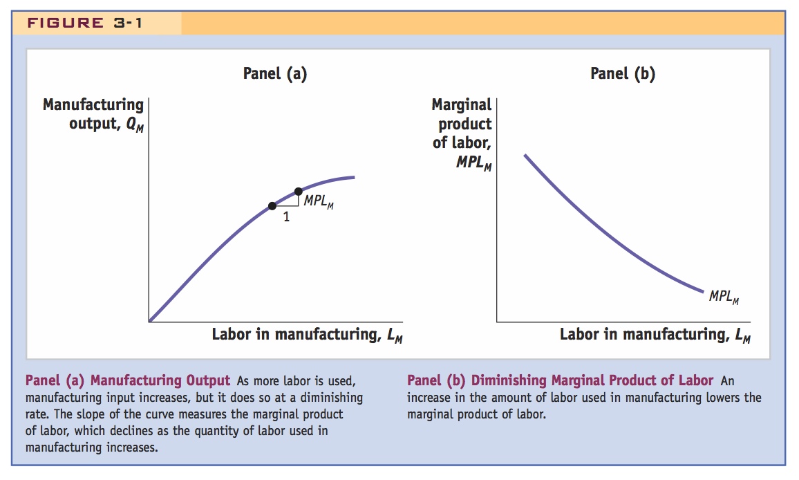
Let us call the two industries in the specific-factors model “manufacturing” and “agriculture.” Manufacturing uses labor and capital, whereas agriculture uses labor and land. In each industry, increases in the amount of labor used are subject to diminishing returns; that is, the marginal product of labor declines as the amount of labor used in the industry increases. Figure 3-1, panel (a), plots output against the amount of labor used in production, and shows diminishing returns for the manufacturing industry. As more labor is used, the output of manufacturing goes up, but it does so at a diminishing rate. The slope of the curve in Figure 3-1 measures the marginal product of labor, which declines as labor increases.
62
Figure 3-1, panel (b), graphs MPLM, the marginal product of labor in manufacturing, against the labor used in manufacturing LM. This curve slopes downward due to diminishing returns. Likewise, in the agriculture sector (not drawn), the marginal product of labor MPLA also diminishes as the amount of labor used in agriculture LA increases.
Be prepared to demonstrate this geometrically.
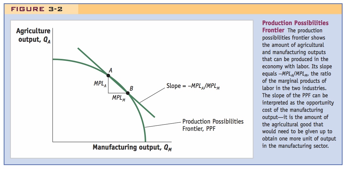
Production Possibilities Frontier Combining the output for the two industries, manufacturing and agriculture, we obtain the production possibilities frontier (PPF) for the economy (Figure 3-2). Because of the diminishing returns to labor in both sectors, the PPF is bowed out or concave with respect to the graph’s origin. (You may recognize this familiar shape from your introductory economics class.)
Note that this is also true in Ricardian model, except that MPs are constant.
By using the marginal products of labor in each sector, we can determine the slope of the PPF. Starting at point A in Figure 3-2, suppose that one unit of labor leaves agriculture and enters manufacturing so that the economy’s new output is at point B. The drop in agricultural output is MPLA, and the increase in manufacturing output is MPLM. The slope of the PPF between points A and B is the negative of the ratio of marginal products, or −MPLA/MPLM. This ratio can be interpreted as the opportunity cost of producing one unit of manufacturing, the cost of one unit of manufacturing in terms of the amount of food (the agricultural good) that would need to be given up to produce it.
Here too, you may need to review. Be prepared to set up a competitive firm's profit max problem and derive the first-order condition.
Opportunity Cost and Prices As in the Ricardian model, the slope of the PPF, which is the opportunity cost of manufacturing, also equals the relative price of manufacturing. To understand why this is so, recall that in competitive markets, firms hire labor up to the point at which the cost of one more hour of labor (the wage) equals the value of one more hour of labor in terms of output. In turn, the value of one more hour of labor equals the amount of goods produced in that hour (the marginal product of labor) times the price of the good. In manufacturing, labor will be hired to the point at which the wage W equals the price of manufacturing PM times the marginal product of labor in manufacturing MPLM.
63
W = PM · MPLM
Observe that this can be rewritten as P = W/MP, which with a little interpretation can be expressed as P = MC (in terms of output). This may be more familiar to some students.
Similarly, in agriculture, labor will be hired to the point at which the wage W equals the price of agriculture PA times the marginal product of labor in agriculture MPLA.
W = PA · MPLA
As in Ricardian, concede that this doesn't happen instantly. However, the stylized fact we invoke here is that it is much harder for land and capital to move than labor.
Because we are assuming that labor is free to move between sectors, the wages in these two equations must be equal. If the wage were not the same in both sectors, labor would move to the sector with the higher wage. This movement would continue until the increase in the amount of labor in the high-wage sector drove down the wage, and the decrease in amount of labor in the low-wage sector drove up the wage, until the wages were equal. By setting the two wage equations equal, we obtain PM · MPLM = PA · MPLA, and by rearranging terms, we get
(PM/PA) = (MPLA/MPLM)
This raises a tricky point that always occurs to some students: If the point of this model is to explain how trade affects DIFFERENT people, what does this indifference curve represent? Who's utility function is it, anyway? The technical answer is that this is a Community Indifference Curve, which presupposes the goods are redistributed so that everybody gets the same utility (this bears upon the case for gains from trade, soon). But at this point it is probably sufficient to wave your hands and say this is way of assessing "overall" welfare.
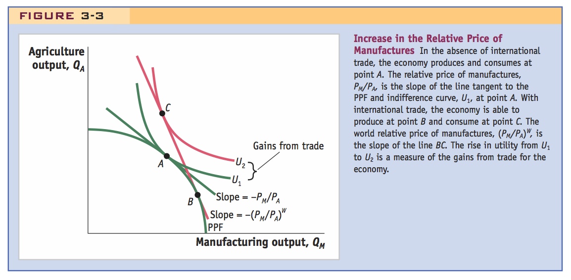
This equation shows that the relative price of manufacturing (PM/PA) equals the opportunity cost of manufacturing (MPLA/MPLM), the slope of the production possibilities frontier. These relative prices also reflect the value that Home consumers put on manufacturing versus food. In the absence of international trade, the equilibrium for the Home economy is at point A in Figure 3-3, where the relative price of manufacturing (PM/PA) equals the slope of the PPF as well as the slope of the indifference curve for a representative consumer with utility of U1. The intuition for the no-trade equilibrium is exactly the same as for the Ricardian model in Chapter 2: equilibrium occurs at the tangency of the PPF and the consumer’s indifference curve. This point on the PPF corresponds to the highest possible level of utility for the consumer.
64
The Foreign Country
Emphasize that in all of these models trade is generated by differences in autarkic relative prices
In this chapter, we do not discuss the Foreign country in any detail. Instead, we simply assume that the no-trade relative price of manufacturing in Foreign  differs from the no-trade price (PM/PA) at Home. There are several reasons why these prices can differ. In the previous chapter, we showed how differences in productivities across countries cause the no-trade relative prices to differ across countries. That is the key assumption, or starting point, of the Ricardian model. Another reason for relative prices to differ, which we have not yet investigated, is that the amounts of labor, capital, or land found in the two countries are different. (That will be the key assumption of the Heckscher-Ohlin model, which we discuss in the next chapter.)
For now, we will not explain why the no-trade relative prices differ across countries but will take it for granted that this is not unusual. For the sake of focusing on one case, let us assume that the Home no-trade relative price of manufacturing is lower than the Foreign relative price, (PM/PA) <; . This assumption means that Home can produce manufactured goods relatively cheaper than Foreign, or, equivalently, that Home has a comparative advantage in manufacturing.
Overall Gains from Trade
Starting at the no-trade equilibrium point A in Figure 3-3, suppose that the Home country opens up to international trade with Foreign. Once trade is opened, we expect that the world equilibrium relative price, that is, the relative price in all countries (PM/PA)W, will lie between the no-trade relative prices in the two countries, so

Given the preceding observation, this follows naturally (except that in Ricardian the inequalities may not be strict).
This equation shows us that when Home opens to trade, the relative price of manufacturing will rise, from (PM/PA) to (PM/PA)W; conversely, for Foreign, the relative price of manufacturing will fall, from to (PM/PA)W. With trade, the world relative price (PM/PA)W is represented by a line that is tangent to Home’s PPF, line BC in Figure 3-3. The increase in the Home relative price of manufactured goods is shown by the steeper slope of the world relative price line as compared with the Home no-trade price line (through point A).
Now the nature of this utility function becomes important. If some people gain and some lose, what does this difference in utility mean? Whose utility?
What this means implicitly is that gainers are compensating losers enough so that they have the same utility, using precisely the kind of redistributive policies that will seem so problematic later.
What is the effect of this increase in (PM/PA) at Home? The higher relative price of the manufactured good at Home attracts more workers into that sector, which now produces at point B rather than A. As before, production takes place at the point along the Home PPF tangent to the relative price line, where equality of wages across industries is attained. The country can then export manufactures and import agricultural products along the international price line BC, and it reaches its highest level of utility, U2, at point C. The difference in utility between U2 and U1 is a measure of the country’s overall gains from trade. (These overall gains would be zero if the relative prices with trade equaled the no-trade relative prices, but they can never be negative—a country can never be made worse off by opening to trade.)
65
In addition to showing the increase in (community) utility, the gains from trade can also be motivated just by noting that trade rotates the budget constraint outside of the PPF: The consumption opportunities set increases, so that there is potentially more to go around for everybody.
A compelling way to make this case is to picture GDP as a pie, the size of which increases with trade.
It is also a good place to explain the notion of Pareto optimality, and argue that trade is a POTENTIAL Pareto improvement.
Notice that the good whose relative price goes up (manufacturing, for Home) is exported and the good whose relative price goes down (agriculture, for Home) is imported. By exporting manufactured goods at a higher price and importing food at a lower price, Home is better off than it was in the absence of trade. To measure the gains from trade, economists rely on the price increases for exports and the price decreases for imports to determine how much extra consumption a country can afford. The following application considers the magnitude of the overall gains from trade in historical cases in which the gains have been measured.
Historical episodes: Thomas Jefferson’s embargo on Britain, 1807–1809 reduced U.S. GDP by 5 percent; Japan’s opening after Perry’s visit in 1854 raised Japanese GDP by about 4 or 5 percent of GDP.
How Large Are the Gains from Trade?
How large are the overall gains from trade? There are a few historical examples of countries that have moved from autarky (i.e., no trade) to free trade, or vice versa, quickly enough that we can use the years before and after this shift to estimate the gains from trade.
One such episode in the United States occurred between December 1807 and March 1809, when the U.S. Congress imposed a nearly complete halt to international trade at the request of President Thomas Jefferson. A complete stop to all trade is called an embargo. The United States imposed its embargo because Britain was at war with Napoleon, and Britain wanted to prevent ships from arriving in France that might be carrying supplies or munitions. As a result, Britain patrolled the eastern coast of the United States and seized U.S. ships that were bound across the Atlantic. To safeguard its own ships and possibly inflict economic losses on Britain, the United States declared a trade embargo for 14 months from 1807 to 1809. The embargo was not complete, however; the United States still traded with some countries, such as Canada and Mexico, that didn’t have to be reached by ship.
As you might expect, U.S. trade fell dramatically during this period. Exports (such as cotton, flour, tobacco, and rice) fell from about $49 million in 1807 to $9 million in 1809. The drop in the value of exports reflects both a drop in the quantity exported and a drop in the price of exports. Recall that in Chapter 2 we defined the terms of trade of a country as the price of its export goods divided by the price of its import goods, so a drop in the price of U.S. exports is a fall in its terms of trade, which is a loss for the United States. According to one study, the cost of the trade embargo to the United States was about 5% of gross domestic product (GDP). That is, U.S. GDP was 5% lower than it would have been without the trade embargo. The cost of the embargo was offset somewhat because trade was not completely eliminated and because some U.S. producers were able to shift their efforts to producing goods (such as cloth and glass) that had previously been imported. Thus, we can take 5% of GDP as a lower estimate of what the gains from trade for the United States would have been relative to a situation with no trade.
Is 5% of GDP a large or small number? It is large when we think that a recession that reduced GDP by 5% in one year would be regarded as a very deep downturn.3 To get another perspective, instead of comparing the costs of the embargo with overall GDP, we can instead compare them with the size of U.S. exports, which were 13% of GDP before the embargo. Taking the ratio of these numbers, we conclude that the cost of the embargo was more than one-third of the value of exports.
66
Another historical case was Japan’s rapid opening to the world economy in 1854, after 200 years of self-imposed autarky. In this case, military action by Commodore Matthew Perry of the United States forced Japan to open up its borders so that the United States could establish commercial ties. When trade was opened, the prices of Japanese exports to the United States (such as silk and tea) rose, and the prices of U.S. imports (such as woolens) fell. These price movements were a terms-of-trade gain for Japan, very much like the movement from the no-trade point A in Figure 3-3 to a trade equilibrium at points B and C. According to one estimate, Japan’s gains from trade after its opening were 4 to 5% of GDP.4 The gains were not one-sided, however; Japan’s trading partners—such as the United States—also gained from being able to trade in the newly opened markets.
The pie shrank by 5 percent.