3 Earnings of Capital and Land
1. Objective:
Explain how trade affects the returns to the specific factors.
2. Determining the Payments to Capital and Land
In each sector, the fixed factor receives a payment equal to the residual of revenue after wage costs. The rental rates (payment per unit of the fixed factor) are in turn equal to the value of the marginal product of each fixed factor: RK = PM • MPKM and RT = PA • MPTM.
a. Changes in the Real Rental on Capital
The rental rate on capital is RK = PM * MPKM. Suppose trade causes PM to increase, labor shifts into manufacturing, which raises MPKM. Therefore RK increases.
Real returns? The real return to capital in terms of manufactured goods RK⁄PM must increase because MPKM has increased. The real return in terms of food RK⁄PA must also increase, since RK has increased and PA is by assumption constant.
Conclusion: Trade unambiguously benefits the owners of capital.
b. Changes in the Real Rental on Land
Symmetrically, trade unambiguously hurts the landowners.
c. Summary
Trade benefits factors specific to the export sector, but hurts factors specific to the import sector.
3. Numerical Example
This section provides a numerical example that verifies the previous theoretical results: Trade causes large changes in the returns to specific factors. However, it causes smaller changes
Let us now return to the specific-factors model. We have found that with the opening of trade and an increase in the relative price of manufactures, there are overall gains for the country, but labor does not necessarily gain. What about the gains to the other factors of production, either the capital used in manufacturing or the land used in agriculture? Capital and land are the two specific factors of production that cannot shift between the two industries; let us now look at the effect of the increase in the relative price of manufactures on the earnings of these specific factors.
Determining the Payments to Capital and Land
In each industry, capital and land earn what is left over from sales revenue after paying labor. Labor (LM and LA) earns the wage W, so total payments to labor in manufacturing are W · LM and in agriculture are W · LA. By subtracting the payments to labor from the sales revenue earned in each industry, we end up with the payments to capital and to land. If QM is the output in manufacturing and QA is the output in agriculture, the revenue earned in each industry is PM · QM and PA · QA, and the payments to capital and to land are
75
Payments to capital = PM · QM − W · LM
Payments to land = PA · QA − W · LA
Rise in Coffee Prices—Great for Farmers, Tough on Co-ops
Services Workers Are Now Eligible for Trade Adjustment Assistance
President Kennedy first introduced Trade Adjustment Assistance (TAA) in the United States in 1962, for workers in manufacturing. This article described how it was extended in 2009 to include service workers. The TAA program was reauthorized by the 2011 U.S. Congress through the end of 2013, and we can expect its continued reauthorization in the future to support workers who are displaced by trade.
In today’s era of global supply chains, high-speed Internet connection, and container shipping, Kennedy’s concerns remain relevant: technology and trade mean growth, innovation and better living standards, but also change and instability. (Research early in this decade typically found that international competition accounted for about 2 percent of layoffs.) But while concerns may be permanent, specific programs and policies fade unless they adapt to changing times. And despite its periodic update, until this week TAA remained designed for an older world. Most notably, it barred support for services workers facing Internet-based competition….
In this context, yesterday’s…bill signing contained the first fundamental change to the TAA program in a half-century. An accord three years in the making, overseen by Senators Max Baucus (D-MT) and Charles Grassley (R-IA), reshapes TAA for the 21st century. The new program, set out in 184 pages of legal text, has three basic changes:
- More workers are eligible: Service-industry employees will be fully eligible for TAA services, making the program relevant to the high-tech economy. So will workers whose businesses move abroad, regardless of the destination. The reform also eases eligibility for farmers and fishermen.
- They get more help: The reform raises training support from $220 million to $575 million, hikes support for health insurance from 65 percent to 80 percent of premiums, gives states $86 million a year to pay for TAA caseworkers, creates a $230 million program to support communities dealing with plant closure, and triples support for businesses managing sudden trade competition.
- They are more likely to know their rights: The bill also creates a special Labor Department TAA office to ensure that eligible workers know their options.
Kennedy’s innovation is thus adapted to the 21st-century economy, guaranteeing today’s workers the support their grandparents enjoyed. A bit of good news, in a year when it is all too rare.
Source: Excerpted from Progressive Policy Institute trade fact of the week, “Services Workers Are Now Eligible for Trade Adjustment Assistance,” February 18, 2009.
It will be useful to take these payments one step further and break them down into the earnings of each unit of capital and land. To do so, we need to know the quantity of capital and land. We denote the quantity of land used in agriculture as T acres and the quantity of capital (number of machines) used in manufacturing as K. Thus, the earnings of one unit of capital (a machine, for instance), which we call RK, and the earnings of an acre of land, which we call RT, are calculated as
76

Economists call RK the rental on capital and RT the rental on land. The use of the term “rental” does not mean that the factory owners or farmers rent their machines or land from someone else, although they could. Instead, the rental on machines and land reflects what these factors of production earn during a period when they are used in manufacturing and agriculture. Alternatively, the rental is the amount these factors could earn if they were rented to someone else over that same time.
There is a second way to calculate the rentals, which will look similar to the formula we have used for wages. In each industry, wages reflect the marginal product of labor times the price of the good, W = PM · MPLM = PA · MPLA. Similarly, capital and land rentals can be calculated as

where MPKM is the marginal product of capital in manufacturing, and MPTA is the marginal product of land in agriculture. These marginal product formulas give the same values for the rentals as first calculating the payments to capital and land, as we just did, and then dividing by the quantity of capital and land. We will use both approaches to obtain rental values, depending on which is easiest.
They may be familiar with the terminology that the two factors are complements in production. This may elicit discussion of when an increase in K, say, might reduce MPL, so the factors are substitutes in production.
Students often confuse these concepts, so it bears emphasis
Change in the Real Rental on Capital Now that we understand how the rentals on capital and land are determined, we can look at what happens to them when the price of the manufactured good PM rises, holding constant the price in agriculture PA. From Figure 3-5, we know that the wage rises throughout the economy and that labor shifts from agriculture into manufacturing. As more labor is used in manufacturing, the marginal product of capital rises because each machine has more labor to work it. In addition, as labor leaves agriculture, the marginal product of land falls because each acre of land has fewer laborers to work it. The general conclusion is that an increase in the quantity of labor used in an industry will raise the marginal product of the factor specific to that industry, and a decrease in labor will lower the marginal product of the specific factor. This outcome does not contradict the law of diminishing returns, which states that an increase in labor will lower the marginal product of labor because now we are talking about how a change in labor affects the marginal product of another factor.
Using the preceding formulas for the rentals, we can summarize the results so far with

That is, the increase in the marginal product of capital in manufacturing means that RK/PM also increases. Because RK is the rental for capital, RK/PM is the amount of the manufactured good that can be purchased with this rent. Thus, the fact that RK/PM increases means that the real rental on capital in terms of the manufactured good has gone up. For the increase in the real rental on capital to occur even though the price of the manufactured good has gone up, too, the percentage increase in RK must be greater than the percentage increase in PM.12
77
The amount of food that can be purchased by capital owners is RK/PA. Because RK has increased, and PA is fixed, RK/PA must also increase; in other words, the real rental on capital in terms of food has also gone up. Because capital owners can afford to buy more of both goods, they are clearly better off when the price of the manufactured good rises. Unlike labor, whose real wage increased in terms of one good but fell in terms of the other, capital owners clearly gain from the rise in the relative price of manufactured goods.
Change in the Real Rental on Land Let us now consider what happens to the landowners. With labor leaving agriculture, the marginal product of each acre falls, so RT/PA also falls. Because RT is the rental on land, RT/PA is the amount of food that can be purchased with this rent. The fact that RT/PA falls means that the real rental on land in terms of food has gone down, so landowners cannot afford to buy as much food. Because the price of food is unchanged while the price of the manufactured good has gone up, landowners will not be able to afford to buy as much of the manufactured good either. Thus, landowners are clearly worse off from the rise in the price of the manufactured good because they can afford to buy less of both goods.
Emphasize this punchline, after all of the preceding derivations.
Summary The real earnings of capital owners and landowners move in opposite directions, an outcome that illustrates a general conclusion: an increase in the relative price of an industry’s output will increase the real rental earned by the factor specific to that industry but will decrease the real rental of factors specific to other industries. This conclusion means that the specific factors used in export industries will generally gain as trade is opened and the relative price of exports rises, but the specific factors used in import industries will generally lose as trade is opened and the relative price of imports falls.
Numerical Example
Break the class into teams. Ask each one to construct its own numerical example and present the calculations to the class. Also assign a numerical example as a homework problem.
We have come a long way in our study of the specific-factors model and conclude by presenting a numerical example of how an increase in the relative price of manufactures affects the earnings of labor, capital, and land. This example reviews the results we have obtained so far using actual numbers. Suppose that the manufacturing industry has the following payments to labor and capital:
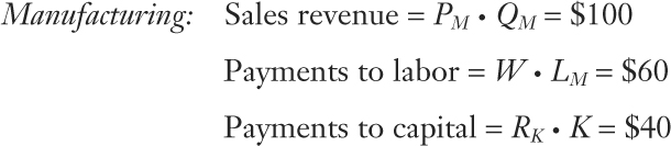
Notice that 60% of sales revenue in manufacturing goes to labor, and 40% goes to capital.
78
In agriculture, suppose that the payments to labor and land are as follows:
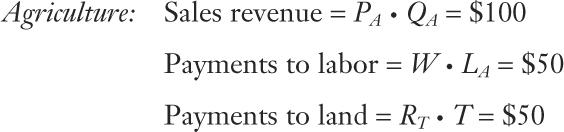
In the agriculture industry, we assume that land and labor each earn 50% of the sales revenue.
An increase in the relative price of manufactures PM/PA can be caused by an increase in PM or a decrease in PA. To be specific, suppose that the price of manufactures PM rises by 10%, whereas the price of agriculture PA does not change at all. We have found in our earlier discussion that ΔW/W, the percentage change in the wage, will be between the percentage change in these two industry prices. So let us suppose that ΔW/W, is 5%. We summarize these output and factor price changes as follows:
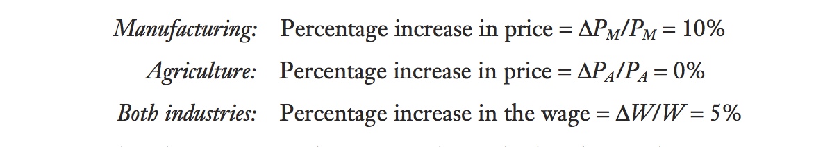
Notice that the increase in the wage applies in both industries because wages are always equalized across sectors.
Change in the Rental on Capital Our goal is to use the preceding data for manufacturing and agriculture to compute the change in the rental on capital and the change in the rental on land. Let’s start with the equation for the rental on capital, which was computed by subtracting wage payments from sales revenue and then dividing by the amount of capital:

If the price of manufactured goods rises by ΔPM > 0, holding constant the price in agriculture, then the change in the rental is

We want to rewrite this equation using percentage changes, like ΔPM/PM, ΔW/W, and ΔRK/RK. To achieve this, divide both sides by RK and rewrite the equation as

You can cancel terms in this equation to check that it is the same as before.
The term ΔPM/PM in this equation is the percentage change in the price of manufacturing, whereas ΔW/W is the percentage change in the wage. Given this information, along with the preceding data on the payments to labor, capital, and sales revenue, we can compute the percentage change in the rental on capital:

79
We see that the percentage increase in the rental on capital, 17.5%, exceeds the percentage increase in the relative price of manufacturing, 10% (so ΔRK/RK > ΔPM/PM > 0). This outcome holds no matter what numbers are used in the preceding formula, provided that the percentage increase in the wage is less than the percentage increase in the price of the manufactured good (as proved in Figure 3-5).
Change in the Rental on Land We can use the same approach to examine the change in the rental on land. Continuing to assume that the price of the manufactured good rises, while the price in agriculture stays the same (ΔPA = 0), the change in the land rental is

Because the wage is increasing, ΔW > 0, it follows immediately that the rental on land is falling, ΔRT <; 0. The percentage amount by which it falls can be calculated by rewriting the above equation as

Using these earlier data for agriculture in this formula, we get

In this case, the land rent falls by the same percentage amount that the wage increases. This equality occurs because we assumed that labor and land receive the same share of sales revenue in agriculture (50% each). If labor receives a higher share of revenue than land, then the rent on land will fall even more; if it receives a lower share, then the rent on land won’t fall as much.
General Equation for the Change in Factor Prices By summarizing our results in a single equation, we can see how all the changes in factor and industry prices are related. Under the assumption that the price of the manufactured good increased but the price of the agricultural good did not change, we have shown the following:

In other words, wages rise but not as much as the percentage increase in the price of the manufactured good; the rental on capital (which is specific to the manufacturing sector) rises by more than the manufacturing price, so capital owners are better off; and the rental on land (which is the specific factor in the other sector) falls, so landowners are worse off.
What happens if the price of the manufactured good falls? Then the inequalities are reversed, and the equation becomes

In this case, wages fall but by less than the percentage decrease in the manufactured good; the rental on capital (which is specific to the manufacturing sector) falls by more than the manufacturing price, so capital owners are worse off; and the rental on land (which is the specific factor in the other sector) rises, so landowners are better off.
80
What happens if the price of the agricultural good rises? You can probably guess based on the previous example that this change will benefit land and harm capital. The equation summarizing the changes in all three factor earnings becomes

Note that it is the specific factor in the agricultural sector that gains and the specific factor in manufacturing that loses. The general result of these summary equations is that the specific factor in the sector whose relative price has increased gains, the specific factor in the other sector loses, and labor is “caught in the middle,” with its real wage increasing in terms of one good but falling in terms of the other. These equations summarize the response of all three factor prices in the short run, when capital and land are specific to each sector but labor is mobile.
What It All Means
This is a nice intuitive explanation that would complement your exposition of the summary in 3.3 Earnings of Capital and Land.
Our results from the specific-factors model show that the earnings of specific factors change the most from changes in relative prices due to international trade. Regardless of which good’s price changes, the earnings of capital and land show the most extreme changes in their rentals, whereas the changes in the wages paid to labor are in the middle. Intuitively, these extreme changes in factor prices occur because in the short run the specific factors are not able to leave their sectors and find employment elsewhere. Labor benefits by its opportunity to move between sectors and earn the same wage in each, but the interests of capital and land are opposed to each other: one gains and the other loses. This suggests that we ought to be able to find real-world examples in which a change in international prices leads to losses for either capitalists or landowners. There are many such examples, and we discuss one in the next application.
As countries become more efficient, agricultural prices fall. The specific-factor model predicts that this will benefit capital, hurt landowners (farmers), and have ambiguous effects on workers. Example of how fluctuations in coffee prices hurt coffee producers in Central America; Fair-Trade Coffee as a form of insurance.
Elaborate on this to say that S-F predicts that volatile world goods prices can induce volatile changes in the distribution of income.
Prices in Agriculture
At the end of the previous chapter, we discussed the Prebisch-Singer hypothesis, which states that the prices of primary commodities tend to fall over time. Although we argued that this hypothesis does not hold for all primary commodities, it does hold for some agricultural goods: the relative prices of cotton, palm oil, rice, sugar, rubber, wheat, and wool declined for more than half the years between 1900 and 1998. Generally, agricultural prices fall as countries become more efficient at growing crops and begin exporting them. From our study of the specific-factors model, it will be landowners (i.e., farmers) who lose in real terms from this decline in the relative price of agricultural products. On the other hand, capital owners gain in real terms, and changes in the real wage are ambiguous. Faced with declining real earnings in the agriculture sector, governments and other groups often take actions to prevent the incomes of farmers from falling.
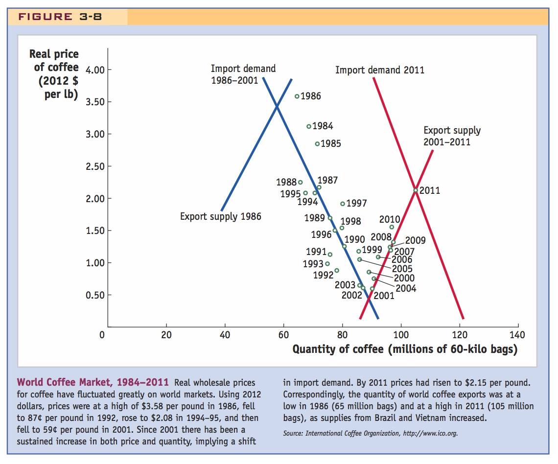
Coffee Prices An example of an agricultural commodity with particularly volatile prices is coffee. The price of coffee on world markets fluctuates a great deal from year to year because of weather and also because of the entry of new suppliers in Brazil and new supplying countries such as Vietnam. The movements in the real wholesale price of coffee (measured in 2012 dollars) are shown in Figure 3-8. Wholesale prices were at a high of $3.58 per pound in 1986, then fell to a low of 87¢ per pound in 1992, rose to $2.08 in 1994–95, and then fell to 59¢ per pound in 2001. Since 2001 there has been a sustained increase in both price and quantity, implying a shift in import demand. By 2011 prices had risen to $2.15 per pound. These dramatic fluctuations in prices create equally large movements in the real incomes of farmers, making it difficult for them to sustain a living. The very low prices in 2001 created a crisis in the coffee-growing regions of Central America, requiring humanitarian aid for farmers and their families. The governments of coffee-growing regions in Central America and Asia cannot afford to protect their coffee farmers by propping up prices, as do the industrial countries.
81
According to the specific-factors model, big fluctuations in coffee prices are extremely disruptive to the real earnings of landowners in coffee-exporting developing countries, many of whom are small farmers and their families. Can anything be done to avoid the kind of boom-and-bust cycle that occurs regularly in coffee markets?
82

Fair-Trade Coffee One idea that is gaining appeal is to sell coffee from developing countries directly to consumers in industrial countries, thereby avoiding the middlemen (such as local buyers, millers, exporters, shippers, and importers) and ensuring a minimum price for the farmers. You may have seen “fair-trade” coffee at your favorite coffeehouse. This coffee first appeared in the United States in 1999, imported by a group called TransFair USA that is committed to passing more of the profits back to the growers. TransFair USA is an example of a nongovernmental organization that is trying to help farmers by raising prices, and the consumer gets the choice of whether to purchase this higher-priced product. In addition to coffee, TransFair USA has been applying its Fair Trade label to imports of cocoa, tea, rice, sugar, bananas, mangoes, pineapples, and grapes.
World coffee prices recovered in 2005, which meant that groups like TransFair USA faced a dilemma: the fair-trade prices that they had guaranteed to farmers were actually less than the world price of coffee. The accompanying article Headlines: Rise in Coffee Prices—Great for Farmers, Tough on Co-ops describes how some farmers were tempted to break their contracts with local co-ops (at fixed, fair-trade prices) to deliver coffee to local middlemen at prevailing world prices. TransFair USA and similar organizations purchase coffee at higher than the market price when the market is low (as in 2001), but in other years (like 2005) the fair-trade price is below the market price. Essentially, TransFair USA is offering farmers a form of insurance whereby the fair-trade price of coffee will not fluctuate too much, ensuring them a more stable source of income over time. By protecting farmers against the boom-and-bust cycle of fluctuating prices, they are able to enjoy greater gains from trade by exporting their coffee. So when you consider buying a cup of fair-trade coffee at your favorite coffeehouse, you are supporting coffee farmers who rely on the efforts of groups like TransFair USA to raise their incomes, and applying the logic of the specific-factors model, all at the same time!